Моделирование и анализ данных
2012. Том 2. № 1. С. 35–50
ISSN: 2219-3758 / 2311-9454 (online)
Application of robust statistics in vibration time histories analysis
Аннотация
Statistical parameters of vibration data distributions provide a remarkable source of information in condition monitoring. The assumption of normality leads to comparatively simple description within the framework of classical statistics. However, due to the presence of outliers and heavy-tailed distributions, this approach is often unacceptable. In such cases, robust methods prove superior. The paper is focused on applying robust statistics in analyzing vibration data dispersion and correlation for the purpose of lifetime consumption estimation. This approach is suitable for large rotating machines operated in an industrial plant environment and characterized by significant influences of control parameters and interference. It is shown that robust meth¬ods yield results that are easier to interpret from both qualitative and quantitative viewpoints. Examples re¬ferring to large steam turbines operated by utility power plants are given; however, certain results can be generalized over a broader class of rotating machines or even diagnostic objects.
Общая информация
Ключевые слова: Robust statistics, vibration analysis
Рубрика издания: Научная жизнь
Тип материала: научная статья
Для цитаты: Gałka T. Application of robust statistics in vibration time histories analysis // Моделирование и анализ данных. 2012. Том 2. № 1. С. 35–50.
Полный текст
1. INTRODUCTION
Vibration-based symptoms are extremely important in monitoring technical condition of virtually all types of rotating machinery, especially large and complex units, e.g. turbo-generators, large fans or compressors. This is justified by their high information content, non-intrusive nature and comparatively well-developed data acquisition and processing procedures. The most straightforward approach consists in analyzing vibration patterns recorded at a certain moment on the basis of a purpose-developed diagnostic model. Information on the object condition is, however, also contained in time histories of certain vibration components. As pointed out in References[1,2], a vibration component evolution type and relevant timescale (the latter varying within a broad range, from seconds to months) contain information on a fault type and thus are useful already at the qualitative diagnosis stage. More detailed analysis of vibration time histories becomes even more important when it comes to quantitative assessment and is mandatory for a prognosis.
Theoretical considerations based on the energy transformation and dissipation processes[3] yield a symptom time history in the form of a continuous, smooth and monotonically increasing function. In practice, however, such approximation may be accepted only for fast-developing faults that strongly influence vibration patterns. More typically, a vibration time history recorded with a real object is an increasing function on which considerable fluctuations are superimposed. An example is shown in Figure 1. Large rotating machines usually generate broadband vibration and relative magnitude of these fluctuations depends on frequency, being substantially larger for so-called blade components, i.e. those produced by interaction between fluid-flow system and medium flow[4].
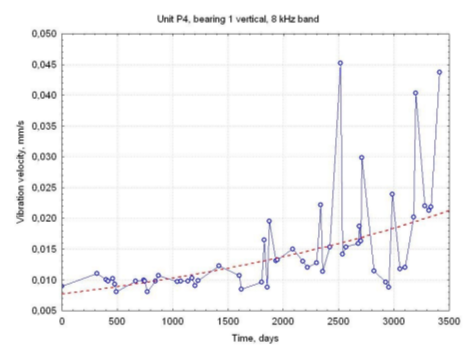
Figure 1. An example of vibration time history: K-200 unit, front high-pressure turbine bearing, vertical direction, 8 kHz band. Dashed line represents exponential fit.
In general, these fluctuations result from the influence of control parameters and interference in accordance with a relation that is fundamental for technical diagnostics:
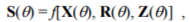
where S, X, R and Z are vectors of symptoms, condition parameters, control and interference, respectively, and в denotes time.
For a given object operated at some fixed location, control and interference parameters may be considered random variables. Therefore, any observable symptom S e S may also be analyzed from the statistical point of view. This has led to the concept of statistical symptoms (or, more precisely, meta-symptoms). In particular, it has been shown[5] that a measure of symptom value dispersion determined within a ‘window’ that is moved along the time axis (see Figure 2) depends on condition parameters and is therefore compliant with the diagnostic symptom definition (this will be dealt with in more detail in Section 3). The approach referred to as the classical one[6] is based on the assumption of approximate normality; hence standard deviation was the first dispersion measure used[7,8]. However, as it is clearly illustrated by Figure1, vibration time histories usually exhibit pronounced outliers and therefore distributions are typically of the heavy-tailed type. In fact, this observation is implicitly contained in results of rather early model considerations, wherein Weibull and Frechet symptom operators have been shown to be applicable13,9]. Elimination of outliers on a basis of some pre-defined criteria is obviously possible[10], but relevant procedures inevitably involve a certain degree of subjectivity.
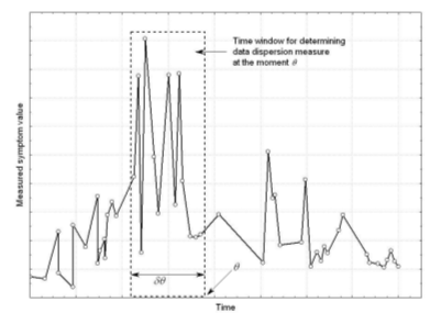
Figure 2. The idea of statistical symptom determination: parameters pertaining to measured symptom value distribution are determined within a time window 86 .
There is thus a need for an approach that would yield reliable estimation of statistical parameters also in the presence of outliers. Such possibility is offered by robust or resistant methods.
2. OBJECTS AND MEASUREMENT DATA
In order not to break up the considerations that will follow, a short description of objects and measurement data acquisition is provided first.
All vibration data have been obtained with large steam turbines operated at utility power plants. Absolute vibration velocity 23% CPB (constant-percentage bandwidth) spectra have been recorded at turbine bearings and casings during steady-state operation. Amplitudes in frequency bands determined on the basis of turbine vibrodiagnostic models[2] are taken as primary vibrationbased symptoms. Steam turbines are designed for an operational life of a few dozen years, so their technical condition evolution is typically slow. Analyzed time histories cover periods up to about fourteen years; in some cases, last measurements were performed shortly before de-commissioning and an ‘accelerated wear’ condition may be expected.
In order to demonstrate the potential of the robust approach, attention has been focused mainly on vibration components from the blade frequency range. As already mentioned, they are characterized by strong influence of control and interference. Moreover, they are not affected by maintenance and minor repairs that do not involve turbine casing opening; therefore, there is no need for symptom normalization, which may be quite tedious and problematic. Frequencies of these components are determined by numbers of stationary and rotating blades in individual turbine stag- es[2,11] and typically cover a range from a few hundred hertz to some 10:20 kilohertz. It has to be kept in mind that detection of these components demands piezoelectric vibration transducers: in typical permanent monitoring systems they are cut off and do not influence total vibration levels, although in some cases are substantially higher in amplitude than low-frequency harmonic components.
3. DISPERSION MEASURES
According to Energy Processor (EP) model[3], information on object condition is contained in the power of residual processes V given in the simplest (linear and stationary) case by
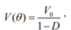
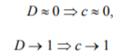
where D = 0/0b, with 0b denoting time to breakdown determined by time-invariant properties of the object, and V0 = V(0 = 0). V is usually non-measurable, hence object condition assessment is based on symptoms, each being related to V by a symptom operator. As already mentioned, control and interference are characterized by random variables with time-invariant distributions. Thus, if it can be shown that

or
then a measure of the dispersion of the V values depends on X and therefore contains information on object condition. It is easily checked that conditions given by Eqs.(3) and (4) for the power of residual processes will also hold for a symptom, irrespective of the symptom operator type.
Suppose for the time being that we deal with a single symptom  and neglect the influence of interference. Moreover, it is assumed that D, that represents object lifetime consumption, is the only condition parameter accounted for; with such approach, D may be viewed as a scalar measure of the vector X. In order to model the influence of control parameters, their vector R is also replaced with a scalar measure. For an energy transforming object, control may be viewed as an operator’s purposeful action aimed at obtaining desired output power; hence it is natural to accept output (or input) power Nu (Ni) as the scalar measure of R. It is more convenient to speak in terms of the input power, keeping in mind that Nu is a monotonic function of Ni. With such assumptions, we finally arrive at the differential equation
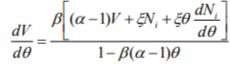
where a, 0 and £ are time-invariant parameters of the object under consideration (details can be found in References[5]). Due to the accumulative nature of the EP model, some form of the Ni(e) function has to be assumed in order to obtain CVlCNi in an analytical form. We may, however, assume that changes of Ni are very slow, so that the dNi/de term in the numerator of Eq.(5) can be neglected. This yields
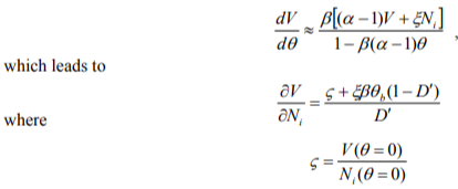
and D' = 1 - D is residual life. The condition given by Eq.(3) is thus fulfilled;  is a monotonically increasing function with the same vertical asymptote as
In general, external and internal interferences are distinguished, depending on whether the source is outside or inside the object. Within the framework of the EP model, only the former can be accounted for. As pointed out in References[4], interference may affect the value of V and hence of S either indirectly, via the energy dissipation processes, or directly. Indirect influence may be treated in the manner similar to outlined above for control, as interference is basically seen as some additional energy supplied to the object. The condition given by Eq.(4) is thus also fulfilled. Direct influence may in turn be identified with the measurement error and it seems reasonable to assume that, with proper data acquisition methods and equipment, it may be minimized to a point of neglecting.
Having shown that a dispersion measure determined in a manner shown schematically in Figure 2 can be accepted as a condition symptom, we must decide which measure should be chosen. The most straightforward choice is obviously standard deviation ст, based on the assumption of approximate normality. Preliminary results have been reported promising[8]; however, standard deviation time histories have been found somehow irregular. Robust alternatives include median absolute deviation about the median m, defined by
m = Med[ 5 - Med(S)] ,
which in fact consists in centering the data around median rather than mean value, so that the above-mentioned assumption is no longer necessary[6]. Other possibility is offered by sample interquartile range q, also known as midspread or middle fifty, given by[12]:
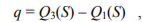


F being the cumulative distribution function. Obviously, for a symmetrical distribution these two approaches are equivalent, but with a heavy-tailed distribution this is not the case. It may also be noted that for the normal distribution both m and q are constant multiples of ст.
It has been noted[8] that time histories of mean absolute difference between consecutive measurements  determined within the time window as in Figure 2 are much more regular and easier to interpret than those of
  . In fact, for all three above dispersion measures it is tacitly assumed that the change resulting from the monotonic trend within the window of the length given by
  is negligible, so that data may be treated in a ‘purely statistical’ manner. This may be accepted only if D is small. It has been pointed out[13] that in analyzing time series one should speak in terms of deviations from the trend rather than from some mean value corresponding to the entire time window. This explains why
  yields better results. Accordingly, yet another symptom may be proposed in the form of
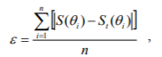
where i is the number of measurements (data points) contained in the time window,  are consecutive symptom value readings and
  represents symptom trend estimated for the entire period under consideration.
Figure 3 presents comparison of results obtained with these five dispersion measures for the symptom time history shown in Figure 1. In order to determine  , exponential trend has been assumed. It is easily seen that all symptoms do increase with time, but
  is obviously strongly influenced by outliers and hence is of ‘step-like’ form. Both m
 and q are far more regular, but certainly
  and are superior; in particular, the latter is most regular and almost perfectly monotonic. The ‘dynamics’ of these symptoms is also noteworthy: during the period covered by observation they increase roughly by one order of magnitude. This is an important advantage. It should be noted that determined on the basis of exponential trend fit in fact cumulates two effects, namely, increasing dispersion and deviation from exponential time history, which becomes substantial for large values of D[7]. It may be inferred that their synergy is responsible for high sensitivity of this symptom to D and results in monotonic and steep time histories. Obviously this is not a disadvantage: sensitivity to condition parameters is in fact an important criterion in choosing most suitable diagnostic symptoms. A question, however, arises whether the above concept works equally well if functions resulting from more appropriate symptom operators have been used (exponential operator is not valid for large values of D).
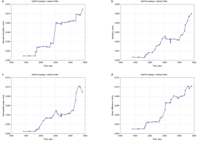
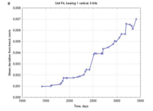
Figure 3. Dispersion measures determined for symptom time history shown in Figure 1; (a) o(0), (b) m(0), (c) q(0), (d) 4(0), (e) s(0). Data window containing 20 points.
Figure 4 shows results obtained with Frechet and Weibull operators. It is easily seen that for both the effect of increasing deviation from trend may be observed; for the Frechet operator the sensitivity to D is only slightly inferior to that achieved with the exponential fit.
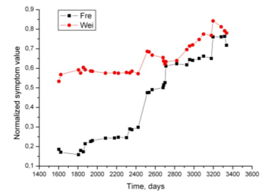
Figure 4. Comparison of s(0) time histories obtained for the case illustrated in Figure 1 with the assumptions of Frechet (Fre) and Weibull (Wei) symptom operators.
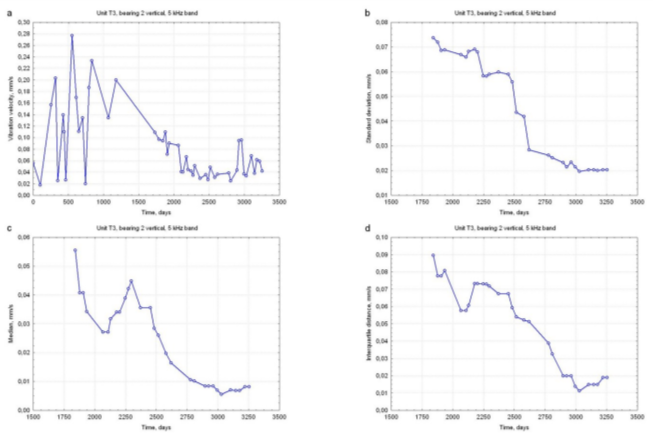
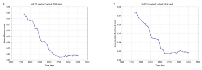
Similar results have been obtained for other turbines, measurement points and frequency bands. It is perhaps worth mentioning here that dispersion measures have also been found appropriate to represent the initial section of the symptom versus time curve, characterized by negative slope (an analogy to the bathtub curve well known from terotechnology and related to the ‘run-in’ process in a broad sense). An example is shown in Figure 5; again,  and
and  prove superior. Handling such case demands certain modifications of basic EP model[5].
Obviously and are not robust dispersion measures and their suitability results from the fact that they account for the presence of a trend within the time window. It seems that a robust measure of deviation from this trend could be developed, which would combine the advantages of these two approaches. It may also be added that still other dispersion estimates have been suggested which might be of use in diagnostic reasoning. An estimate similar to (in the sense that it is based on differences between consecutive measurements) has been proposed[14]. Another possibility of quantifying dispersion is offered by estimates based on the shortest interval that contains at least half of the data, somehow descriptively termed ‘the shortest half’[15]; they have been described as quite promising in terms of robustness.
|
Figure 5. 230 MW unit, rear high-pressure turbine bearing, vertical direction, 5000 Hz band. (a) symptom time history, (b) a(0), (c) m(0), (d) q(0), (e) J(0), (f) s(0). Data window containing 20 points. |
4. MEASURES OF CORRELATION
Following Karl Pearson, a measure of correlation may be referred to as ‘a computational index used to measure bivariate association’[16].The most commonly used quantitative measure of correlation between random variables S1 and S2 is Pearson product-moment correlation coefficient r given by the normalized covariance
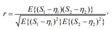
where E denotes expected value and
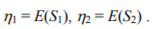
The main deficiency of this coefficient is that it assumes a linear relation between S1 and S2. The second disadvantage results from the fact that r is based on estimated standard deviation and is thus sensitive to outliers. Both these drawbacks may be eliminated or at least alleviated to some extent by using non-linear and more robust measures of correlation. These include the Kendall rank correlation coefficient  given by[17]
In both formulae, N is the number of scores (elements) in two data samples,  denotes symmetric difference distance and di refers to differences between individual ranks. It should be noted here that both
  are calculated on the basis of ranks rather than standard deviations and therefore more suitable for analyzing time series.
Application of correlation measures in condition monitoring is twofold. First, the very existence of correlation is useful in diagnosing certain malfunction types, i.e. in qualitative diagnostics. Second, it has been suggested that evolution of correlation measures with time may be employed in lifetime consumption assessment, i.e. for the quantitative diagnosis.
One of the symptom types listed in References[2] is termed correlation of vibration amplitudes with operational parameters. Although not stated explicitly, this is in fact based on a ‘binary’ approach: correlation is either present or not or, to put it less categorically, is ‘strong’ or ‘weak’. Such concept tacitly implies that strong correlation is viewed indicative of deterministic dependence. Correlation with load or temperature is employed in detecting faults like rotor crack[19] or rub[20]. In what follows, however, attention will be focused on correlation between two vibration-based symptoms.
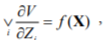
In general, any symptom will depend on a number of condition parameters, so that we cannot speak in terms of deterministic functional relations of the Si = f(Xj) type. We may, however, expect a stochastic relation, which means that changes of Xj will affect probability distribution of Si. Moreover, it seems justified to assume that if
and Xj changes substantially, then with various values of  will fluctuate about some expected value
  This means a statistic or correlative relation. Thus, if two symptoms can be shown to be correlated, we may infer that they are dependent, i.e. that their changes have been caused by the same condition parameter.
Application of correlation measures to fault identification has been dealt with in an earlier study by the author[21] and here we shall aim at determining whether robust approach brings about any improvement. The first example is for a somehow untypical case of the 4xf0 component increase as a result of turbine fluid-flow system failure. Table 1 lists Pearson, Kendall and Spearman coefficients of correlation between this component and those from the lower part of the blade frequency range, for three different turbines of the same type. Two cycles for the (faulty) unit T9 refer to periods before and after repair, respectively. It is easily seen that with the fault present correlation is strong and positive, while in all other cases it is much weaker and some coefficient values are negative. Qualitative conclusions do not depend on which correlation measure has be applied.
The second example refers to intermediate-pressure permanent rotor bow in two turbines. In general, rotor bow produces unbalance, and suitable procedures must employed in order to distinguish from other malfunctions that give similar changes of vibration patterns. It has been shown[21] that permanent bow results in an increased 1xf0 component in axial direction, so strong correlation with this component in vertical direction should be expected. Table 2 lists coefficients determined for five similar turbines of the same general layout; in the case of the faulty units (T1 and T2) consecutive cycles have been determined by rotor balancing, which reduces vertical vibration to an acceptable level, but obviously does not eliminate the root cause (1xf0 component time history for one of the faulty units is shown in Figure 6). Conclusions concerning suitability of various correlation measures are the same as for the previous case: it is evident that robust measures offer no significant advantage. Similar results have been arrived at in other studies by the author[22].
Table 1. Correlation coefficients for units T8, T9 and T10: rear intermediate-pressure turbine bearing, axial direction.
|
Unit and cycle |
Coefficient type |
Coefficie with vi |
nt of correlation of the 4xf0 co bration amplitudes in the banc |
mponent s [Hz] |
||
|
800 |
1000 |
1250 |
1600 |
2000 |
||
|
Unit T8 all |
r |
0.110 |
0.110 |
0.097 |
0.198 |
-0.013 |
|
T |
0.058 |
0.091 |
0.086 |
0.167 |
0.036 |
|
|
p |
0.091 |
0.136 |
0.114 |
0.245 |
0.066 |
|
|
Unit T9 cycle 1 |
r |
0.912 |
0.931 |
0.833 |
0.794 |
0.689 |
|
T |
0.511 |
0.538 |
0.318 |
0.439 |
0.336 |
|
|
p |
0.674 |
0.702 |
0.449 |
0.599 |
0.470 |
|
|
Unit T9 cycle 2 |
r |
-0.009 |
-0.461 |
-0.078 |
-0.060 |
-0.100 |
|
T |
-0.037 |
-0.302 |
-0.032 |
0.041 |
-0.006 |
|
|
p |
-0.029 |
-0.412 |
-0.040 |
0.077 |
-0.030 |
|
|
Unit T10 all |
r |
0.103 |
0.127 |
0.071 |
-0.211 |
-0.206 |
|
T |
0.227 |
0.104 |
0.123 |
-0.257 |
-0.080 |
|
|
p |
0.359 |
0.161 |
0.178 |
-0.390 |
-0.128 |
|
Table 2. Coefficients of correlation between 1xf0 components for five turbines.
|
Unit and cycle |
Coefficient type |
Coefficient of correlation of the 1xf0 component, bearing 3 vertical, with 1xf 0 at |
||
|
bearing 2 axial |
bearing 3 axial |
bearing 4 axial |
||
|
Unit T1 cycle 1 |
r |
0.690 |
0.904 |
0.911 |
|
T |
0.350 |
0.783 |
0.793 |
|
|
p |
0.524 |
0.910 |
0.924 |
|
|
Unit T1 cycle 2 |
r |
0.937 |
0.966 |
0.895 |
|
T |
0.835 |
0.839 |
0.741 |
|
|
p |
0.960 |
0.957 |
0.868 |
|
|
Unit T2 cycle 1 |
r |
0.967 |
0.971 |
0.952 |
|
T |
0.801 |
0.862 |
0.846 |
|
|
p |
0.947 |
0.961 |
0.950 |
|
|
Unit T2 cycle 2 |
r |
0.651 |
0.595 |
0.506 |
|
T |
0.538 |
0.407 |
0.363 |
|
|
p |
0.688 |
0.569 |
0.508 |
|
|
Unit T2 cycle 3 |
r |
0.949 |
0.860 |
0.849 |
|
T |
0.835 |
0.607 |
0.630 |
|
|
p |
0.952 |
0.774 |
0.797 |
|
|
Unit T3 all |
r |
0.569 |
0.405 |
0.308 |
|
T |
0.087 |
0.315 |
0.233 |
|
|
p |
0.137 |
0.423 |
0.320 |
|
|
Unit P3 all |
r |
0.269 |
-0.163 |
-0.490 |
|
T |
0.093 |
-0.168 |
-0.366 |
|
|
p |
0.152 |
-0.237 |
-0.547 |
|
|
Unit P5 all |
r |
0.283 |
0.309 |
-0.082 |
|
T |
0.183 |
0.232 |
-0.127 |
|
|
p |
0.319 |
0.333 |
-0.174 |
|
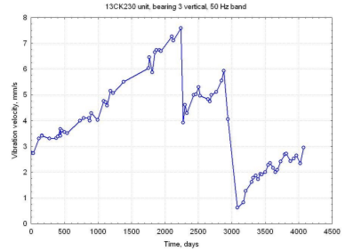
Figure 6. Vibration time history: rear intermediate-pressure turbine bearing, vertical direction, 1xf0 component; permanent rotor bow. Stepwise decreases have been caused by rotor balancing.
4.2. Quantitative diagnosis
The EP model assumes deterministic influence of D on symptom values, so for any  is a monotonically increasing function. In view of Eqs.(2) and (7), as D approaches unity, both Si and
  tend to infinity, so equal increments of D will result in increasing increments of Si:

and this will hold for all symptoms. Correlation between any two symptoms Sj and Sk is thus expected to increase, as both will, to a growing extent, be dominated by D rather than other factors and thus become more deterministic with respect to D. This phenomenon has been termed the ‘Old Man Syndrome’(10). If D is taken as the sole condition parameter and c is a correlation measure  we may infer that
(it is assumed that for every  is a monotonically increasing function of D, so that c should tend to its positive limit). This means that, from the formal point of view, a measure of correlation is conformant with a diagnostic symptom definition and hence can be applied as such. Application of such measure in quantitative diagnostics at the present stage is expected to provide a warning when generalized damage becomes high enough to justify some action, like e.g. rescheduling overhauls or planning purchase of spares.
As pointed out in References[10], suitability of the ‘Old Man Syndrome’ concept in quantitative diagnostics should be first tested on vibration-based symptoms pertaining to the fluid-flow system condition. A period between two consecutive major overhauls can be then considered a single life cycle; for steam turbines this means that, in practice, data covering a dozen or so years may be available. The problem of selecting symptoms with the highest information contents may be solved with the aid of Singular Value Decomposition (SVD) method[10,23].
It has already been mentioned that in analyzing time histories a ‘mean value’ becomes somehow ‘abstract’, especially if the time window is long or D is close to 1. This has led to a suggestion of applying a correlation measure similar to Pearson coefficient (see Eq.(13)), but determined by differences from trends rather than means[10]. Such measure has been tentatively termed ‘modified Pearson coefficient’ r'. Using the notation from Eq.(12), r' is given by
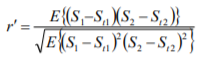
Formally speaking, r' is not a robust measure, as it is also sensitive to outliers; it seems, however, interesting to include it for comparison.
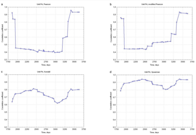
The first example refers to an unit already dealt with (Figures 1, 3 and 4), but different frequency bands (front high-pressure turbine bearing, vertical direction, 5000 Hz and 6300 Hz bands). Figure 7 shows time histories of all four correlation measures introduced earlier in this Section  , for time window containing 25 consecutive data points. It is easily seen that both (r,
  and
and  are characterized by comparatively high initial values that promptly decrease to about 0.35. Influence of some interference that had acted on both symptoms in a similar manner may be suspected. Terminal increasing section is rather short and stepped - obviously outliers are responsible. Introduction of r' brings about only small improvement. On the contrary, both т(в) and р(в) are much more regular and initial high values are absent. Moreover, there is a slight decrease starting at about 2500 days, which can be hardly noticed for r and r'; it has been revealed that this was caused by a repair which de-correlated the symptoms to a certain extent. Final increasing section starts at about 3000 days, which means that an alert is provided with a lead of about two years: a very satis-
factory result indeed, as there should be enough time for a remedial action. On the basis of these results it is clear that the robust approach is superior; both robust coefficients lead to similar conclusions and none can be pointed out as better than the other. Higher values of the Spearman coefficient are typical[6].
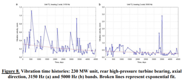
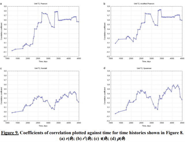
It has been pointed out that the ‘Old Man Syndrome’ can be observed only for old units that are approaching service life end. In fact, in the above example high-pressure turbine rotor was replaced shortly after the last measurement. Figure 8 shows time histories for two symptoms recorded at the rear high-pressure turbine bearing of a 230 MW unit, first measurement having been performed shortly after commissioning. In both cases there is a very weak decreasing tendency with significant outliers. Time histories of correlation coefficients are shown in Figure 9. It is immediately seen that Pearson and modified Pearson coefficients plots (Figure 9a and b) are very similar, even quantitatively; this is hardly surprising, as trends are in both cases very weak.  time histories are quite irregular and obviously heavily influenced by outliers. By contrast, Kendall and Spearman coefficient plots (Figure 9c and d) are much ‘smoother’ and both reveal initial increasing section followed by a sharp drop and then the same sequence again; maximum values are, however, significantly lower than those shown in Figure 7. Just as in previous example, both drops are due to overhauls that de-correlate the symptoms to a substantial degree. Due to the influence of outliers, this effect is hardly noticeable in the plots. Thus, again, robust approach yields results that are much easier to interpret.
Finally, it may be mentioned that other approaches to quantifying correlation have also been proposed, including Renyi maximal correlation[24] and an interesting concept of Pearson correlation derivatives[25]. Their suitability for diagnostic applications and possible advantages still remain to be studied. More recently reported measures employing Brownian or distance correlation[26], will possibly open a promising field for further research.
5. CONCLUSIONS
To quote John W. Tukey, ‘it is perfectly proper to use both classical and robust/resistant methods routinely, and only worry when they are different enough to matter’[27]. It seems reasonable to state that, when dealing with correlation for the purpose of a qualitative diagnosis, i.e. determining whether it is strong or weak, these differences are negligible and conclusions drawn with both classical and robust measures are similar. If, however, dispersion or especially correlation is analyzed as a function of time for the purpose of a quantitative diagnosis and prognosis, robust approach yields significantly better results. Clearly, it is better suited to analyze time histories characterized by strong influences of control and interference. Of particular importance for possible applications, robust approach is capable of providing an ‘early warning’ with considerable lead; this demonstrates that meta-symptoms based on robust measures are highly sensitive to technical condition deterioration.
Acknowledgements
Some of the results used and quoted in this paper have been obtained with the support of the Ministry of Science and Higher Education within the frame work of the N504 030 32/2693 Research Project. The author wishes to express his gratitude to Prof. Stanislaw Radkowski for fruitful discussion that has been very helpful in giving this paper its final form.
Литература
- Morel J., “Vibration des Machines et Diagnostic de Leur État Mécanique”, Eyrolles, Paris, France, 1992.
- Orłowski Z., “Diagnostics in the Life of Steam Turbines”, WNT, Warszawa, Poland, 2001 (in Polish).
- Natke H. G. and Cempel C., “Model-Aided Diagnosis of Mechanical Systems”, Springer, Ber-lin-Heidelberg-New York, 1997
- Gałka T., “Influence of Load and Interference in Vibration-Based Diagnostics of Rotating Machines”, Advances and Applications in Mechanical Engineering and Technology, Vol 3, No 1, pp 1-19, 2011.
- Gałka T. and Tabaszewski M., “An Application of Statistical Symptoms in Machine Condition Diagnostics”, Mechanical Systems and Signal Processing, Vol 25, No 1, pp 253-265, 2011.
- Maronna R. A., Martin R. D. and Yohai V. J., “Robust Statistics”, Wiley, Chichester, UK, 2006
- Gałka T., “Diagnostics of the steam turbine fluid-flow system condition on the basis of vibration trends analysis”, Proceedings of the 7th European Conference on Turbomachinery, Athens, Greece, pp 521-530, March 2007.
- Gałka T., “Statistical Vibration-Based Symptoms in Rotating Machinery Diagnostics”, Diagnostyka, Vol 2, No 46, pp 25-32, 2008.
- Gałka T., “Application of Energy Processor Model for Diagnostic Symptom Limit Value Determination in Steam Turbines, Mechanical Systems and Signal Processing”, Vol 13, No 5, pp 757-764, 1999.
- Gałka T., “The ‘Old Man Syndrome’ in machine lifetime consumption assessment”, Proceedings of the CM2011/MFPT2011 Conference, Cardiff, UK, paper No 108, June 2011.
- Gałka T., “Assessment of the turbine fluid-flow system condition on the basis of vibration-related symptoms”, Proceedings of the 16th International Congress COMADEM 2003, Växjö University, Sweden, pp 165-173, August 2003.
- Upton G. and Cook I., “Understanding Statistics”, Oxford University Press, UK, 1996.
- Aldrich J., “Correlations Genuine and Spurious in Pearson and Yule”, Statistical Science, Vol 10, No 4, pp 364-376, 1995.
- Rousseeuw P. J. and Croux C., “Alternatives to Median Absolute Deviation”, Journal of the American Statistical Association, Vol 88, pp 1273-1283, 1993.
- Martin R. D. and Zamar R. H., “Bias Robust Estimates of Scale”, The Annals of Statistics, Vol 21 pp 991-1017, 1993.
- Rodgers J. L. and Nicewander W. A., “Thirteen Ways to Look at the Correlation Coefficient”, The American Statistician, Vol 42, No 1, pp 59-66, 1988.
- Abdi H., “The Kendall Rank Correlation Coefficient”, in “Encyclopedia of Measurement and Statistics”, N Salkind (Ed.), Sage, USA, 2007.
- Scheaffer R. L. and McClave J. T., “Probability and Statistics for Engineers”, PWS-KENT Publishers, Boston, USA, 1986.
- Bachschmid N., Pennacchi P. and Tanzi E., “Cracked Rotors. A Survey on Static and Dynamic Behaviour Including Modelling and Diagnosis”, Springer, Berlin, Germany, 2010.
- Bently D. E. and Hatch C. T., “Fundamentals of Rotating Machinery Diagnostics”, Bently Pressurized Bearing Press, Minden, USA, 2002.
- Gałka T., “Correlation-based symptoms in rotating machines diagnostics”, Proceedings of the 21st International Congress COMADEM 2008, Praha, Czech Republic, pp 213-226, 2008.
- Gałka T., “Correlation Analysis in Steam Turbine Malfunction Diagnostics”, Diagnostyka, Vol 2, No 54, pp 41-50, 2010.
- Gałka T., “Application of the Singular Value Decomposition method in steam turbine diagnostics”, Proceedings of the CM2010/MFPT2010 Conference, Stratford-upon-Avon, UK, paper No 107, 2010.
- Sethuraman J., “The Asymptotic Distribution of the Rênyi Maximal Correlation”, Florida State University Technical Report No M-835, 1990.
- Strickert M., Schleif F-M., Seiffert U. and Villmann T., “Derivatives of Pearson Correlation for Gradient-Based Analysis of Biomedical Data”, Revista Iberoamericana de Inteligencia Artifical, Vol 12, No 37, pp 37-44, 2008.
- Székely G. J. and Rizzo M. L., “Brownian Distance Covariance”, The Annals of Applied Statistics, Vol 3, No 4, pp 1236-1265, 2009.
- Tukey J. W., “Useable resistant/robust techniques of analysis”, Proceedings of the First ERDA Symposium, Los Alamos, USA, pp 11-31, 1975.
Информация об авторах
Метрики
Просмотров
Всего: 916
В прошлом месяце: 2
В текущем месяце: 2
Скачиваний
Всего: 403
В прошлом месяце: 0
В текущем месяце: 0