Моделирование и анализ данных
2012. Том 2. № 1. С. 59–69
ISSN: 2219-3758 / 2311-9454 (online)
Acoustic characterization of the conditions of a water-filled siphon
Аннотация
Pattern recognition has been used and developed as a process of advanced analysis of acoustic signal. Designing a robust pattern recognition system involves three fundamental tasks: signal pre-processing, feature extraction and selection, and finally classifier design and optimization. This paper reports on an application to detect and monitor conditions of a large, water-filled siphon used in underground tunnels. Acoustic signals were collected from 4 hydrophones under various typical siphon conditions and used as input data to study the variation of the acoustic field. The discrete wavelet transform (DWT) was used in feature extraction and K-nearest neighbors (KNN) classification was applied. Subsequently, the system was tested on new unknown data and compared with supervised training samples. The results demonstrated that the acoustic sensors have high reproducibility for collecting signals under operational conditions. The pattern recognition system is also capable of discriminating different pipe conditions but further refinement is needed to improve sensitivity and to compensate for the effect of variable water level and sensor misalignment.
Общая информация
Ключевые слова: Acoustics, siphon, wavelet transform, pattern recognition
Рубрика издания: Научная жизнь
Тип материала: научная статья
Для цитаты: Feng Z., Horoshenkov K., Noras J. Acoustic characterization of the conditions of a water-filled siphon // Моделирование и анализ данных. 2012. Том 2. № 1. С. 59–69.
Полный текст
1. INTRODUCTION
Acoustics is used widely to determine the conditions of hidden assets, which include pipes, pumping stations and tunnels. It is popular because sound waves provide a rapid, effective and non- invasive means for asset quality control. Historically, Fourier transform-based spectral analysis methods have been used to analyse the collected acoustic data. These are based on time series data processing and calculating global energy-frequency distributions and power spectra. However, the use of Fourier spectral analysis is always limited to linear and stationary systems. In order to overcome these issues, methods of time-frequency analysis, including short-time Fourier transform (STFT), Wigner-Ville Distribution (WVD)[3] and Wavelet Transform (WT)[2], have been recently introduced.
In this analysis it is important to be able to determine patterns which are associated with particular system states. For many industrial applications, identifying and classifying patterns and extracting features using time-series data constitute an important topic for research. In this research a subset of patterns which represents a range of typical conditions is of a particular interest. Feature extraction and pattern recognition algorithms have been developed and used for analysing signals and for signal classification[8] These techniques include hidden Markov models (HMM), K-nearest neighbours (KNN)[5], decision trees, and neural networks methods[4]. Although these techniques found applications in areas related to voice and speech recognition, image analysis and security, they have not been used extensively for the condition monitoring of civil engineering assets. Therefore, this project concentrates on developing a new methodology for the analysis of acoustic data collected in a hydraulic siphon. The aim of this project is to develop a robust classification technique to discover a relationship between the acoustic data and a range of classified patterns obtained for a full-scale model of a hydraulic siphon used in London Underground.
2. EXPERIMENTS SET UP AND DATA COLLECTION
Acoustic data were collected in a siphon which was constructed from 450mm diameter concrete pipes in the Hydraulics Laboratory in the University of Bradford. The siphon was 4.2 m long and 2.0 m high. It was installed on a 500 mm layer of fine sand in an open top box made of 12mm plywood. The siphon was instrumented with four 25 mm hydrophones, 3 of which were installed in the left leg of the siphon. The other hydrophone was installed in the right leg of the siphon 75 mm above the speaker and used as a reference receiver. The source was a 50 mm diameter water resistant speaker in a PVC enclosure which is able to operate underwater. The hydrophones and the speaker were attached securely to two aluminum tubes which were lowered into the opposite legs of the siphon and kept at the same positions in all of the experiments conducted in the siphon. Figure 1 illustrates the equipment used in this experiment. The siphon was filled with clean water to the level of 900 mm below the top of the right vertical pipe (reference water level) in all the experiments except water level test.
The data acquisition and signal processing facilities used in these experiments consisted of: (i) a computer with WinMLS software to control the sound card which generated a sinusoidal sweep in the frequency range of 100 - 6000 Hz; (ii) an 8-channel high-pass hydrophone filter used to remove unwanted low-frequency noise produced by equipment and machinery operated in the laboratory from the signals received on hydrophone H1-H3; (iii) a measuring amplifier and a filter which were used to condition and filter the signal received on the reference hydrophone in the 100 - 4000 Hz range. In addition, a power amplifier was used to drive the underwater speaker. Stereo amplifier and headphones were used to control subjectively the quality of the signal produced by the underwater speaker.
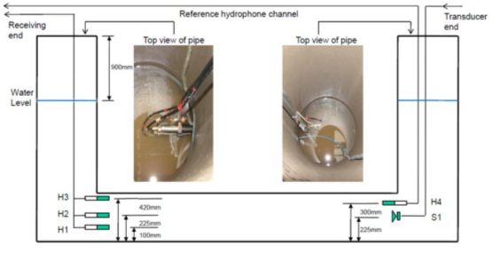
Figure 1. Structure of siphon and sensors
3. SIGNAL PROCESSING METHODOLOGY
For most industrial applications, a classical pattern recognition system consists of the following components: pre-processing, feature extraction, feature selection and pattern classification (decision making). Feature extraction and recognition methods are very important factors to achieve robust system performance. In this work we used the wavelet decomposition and K-nearest neighbors method to analyze the collected acoustic data and classify patterns.
3.1. Wavelet Decomposition
The wavelet transform (WT) is an important part of pre-processing and feature extraction phases in a pattern recognition system. It has been designed to analyze the temporal and spectral properties of non-stationary signals and overcomes the shortcomings of Fourier transform by applying adjustable window to achieve the required frequency and temporal resolution. Applications of 1-D discrete wavelet transform are numerous in acoustical signal processing[1]. A discrete wavelet transform (DWT) decomposes a signal into mutually orthogonal set of wavelets. The signal to be analyzed is passed through filters constructed by a mother wavelet with different cut-off frequencies and at different scales. A discrete wavelet transform of a discrete time signal f(t) with length N and finite energy can be written as:
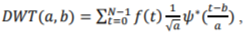
where  defines the family of wavelet function, with
  the scale of the transform and b the spatial (temporal) location, * denotes the complex conjugate.
The process of discrete wavelet transform implemented at each stage can be simplified as low-pass filtering of the signal for the approximations and high-pass filtering of the signal for the details, and then down sampling by half. Filtering a signal corresponds to the convolution of the signal with the impulse response of the filter. The output coefficients can be then expressed mathematically as:
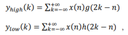
where  are the outputs of the high-pass filter and low-pass filter , respectively, after down sampling by half.
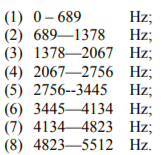
For many signals, it is the low-frequency components which are mostly important. These components define the signal its identity. The wavelet decomposition process can be iterated, with successive approximations being decomposed in turn, so that one signal is broken down into many lower-resolution components. It is called the wavelet decomposition tree[7] as presented in Figure 2.
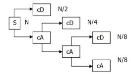
Figure 2. Wavelet decomposition tree
The coefficients vectors and can be then used to reconstruct real filtered signals by reversing the decomposition process. The process yields reconstructed approximations , and details which are true constituents of the original signal, so the original signal can be obtained by combining details and approximations .
3.2. K-nearest neighbors (KNN) method
K-nearest neighbors is a common classification technique based on the use of distance measures. For a given unlabeled sample , find the “closest” labeled samples in the training data set and assign to the class that appears most frequently within the -subset. is the number of considered neighbors. Usually Euclidean distance is used and it is expressed as:
where  is the training data set:
  A typical procedure for the KNN classification process is:
1) Calculate Euclidean distances of all training data to testing data.
2) Construct a new matrix which elements are Euclidean distances between testing data and corresponding training data.
3) Pick K number of samples closest to the testing data by choosing smallest values of Euclidean distance. Larger value of K yields smoother decision regions and, therefore, results in a better classification. However, this increases computational burden as further samples are taken into account.
4) Classification: majority vote. K preferably odd to avoid ties.
4. EXPERIMENTAL CONDITIONS
The acoustic signals recorded in the siphon at two different conditions were decomposed by applying discrete wavelet transform. These conditions were: (i) clean siphon; (ii) siphon with a controlled amount of blockage. The blockage was simulated with bags of sand. Each of this bags contained approximately 1 kg of fine sand. A maximum of 10 bags were used in these experiments.
Signals with the frequency components higher than 5512Hz were filtered out and low-pass f
signals were decomposed into 8 frequency bands with each bandwidth equals to 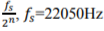 is the sampling frequency, is the depth of the decomposition.
The frequency bands on the 5th depth were calculated as follows:

Therefore, the frequency bands obtained with this method were:
This process can be illustrated with a decomposition tree shown in Figure 3.
Note: 8 frequency bands are presented as their index numbers in brackets as displayed above in the following contents.
Figure 3. Modified wavelet decomposition tree generated by MATLAB
4.1. Reproducibility test
Figure 4 is an example of the acoustic signal from two blockages in the siphon decomposed into 8 filtered signals by using discrete wavelet transform. This process was repeated on at least 3 signals which were collected under the same siphon condition but at different times so that the reproducibility of this experiment could be determined.
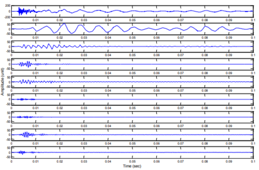
Figure 4. Acoustic impulse response of the siphon with 2 blockages decomposed using sym4 (Singh & Tiwari, 2006) as mother wavelet. From top to bottom: the original signal plus 8 wavelet outputs with a progressive increase in the frequency band.
Energy and cross-correlation coefficients were calculated to describe the similarity between signals at same frequency range. The energy contained in each signal was calculated according to
As the energy of the sound generated by the speaker had varied slightly between individual measurements, the energy percentage in each frequency band was calculated to enable a comparison between these signals

The cross-correlation coefficients were also calculated as
where f(x) is the probability function. The maximum deviation  , where
  represents all samples and
  is the mean of them. Maximum deviation sensitivity C (%) is calculated as a measure of system reliability, the lower value of C indicates more stability of the system
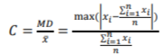
Table 1 presents the result for acoustic energy obtained from the reproducibility test for the siphon blocked with two sand bags. The number in brackets in the top row corresponds to the WT band defined in the above paragraph. This table also presents the maximum deviation sensitivity C (%) which corresponds to the similarity between the data obtained in reproducibility experiments.
Table 1. Acoustic energy percentage of 2 blockages in the siphon at 8 frequency bands and maximum deviation sensitivity.
|
Energy (%) |
(1) |
(2) |
(3) |
(4) |
(5) |
(6) |
(7) |
(8) |
|
Test 1 |
18.61 |
11.97 |
2.18 |
1.20 |
0.49 |
1.33 |
1.55 |
1.15 |
|
Test 2 |
20.14 |
11.76 |
2.30 |
1.21 |
0.47 |
1.35 |
1.58 |
1.13 |
|
Test 3 |
20.83 |
11.29 |
2.17 |
1.09 |
0.50 |
1.37 |
1.56 |
1.10 |
|
C(%) |
6.29 |
3.28 |
3.76 |
6.57 |
3.42 |
1.48 |
1.07 |
2.37 |
Table 2 presents the cross-correlation coefficient obtained in three experiments repeated in the siphon with the same amount of sediment. This table together with the acoustic energy data presented in Table 1 illustrates a very high similarity between the three repeated tests and reproducibility in the experiment.
Table 2. Cross-Correlation coefficients of reproducibility tests of 2 blockages in the siphon
|
Cross-correlation coefficients |
(1) |
(2) |
(3) |
(4) |
(5) |
(6) |
(7) |
(8) |
|
Test 1 VS Test 2 |
0.9989 |
0.9995 |
0.9992 |
0.9983 |
0.9961 |
0.9988 |
0.9991 |
0.9992 |
|
Test 1 VS Test 3 |
0.9993 |
0.9996 |
0.9989 |
0.9991 |
0.9997 |
0.9990 |
0.9993 |
0.9969 |
|
Test 2 VS Test 3 |
0.9985 |
0.9991 |
0.9976 |
0.9988 |
0.9979 |
0.9991 |
0.9994 |
0.9980 |
4.2. Condition classification
The values of acoustic energy and correlation coefficients calculated for 8 WT bands were used as features to construct a training data matrix. The same process was repeated on the acoustic signals collected from unknown pipe condition and testing data matrix was constructed in the same way (see Table 3 and 4). Both matrices were used with K-nearest neighbors algorithm to determine the condition of the siphon from new testing data. The value of K was chosen 1 so that only the nearest neighbor from the training data could be found. Examples of blockage condition matrices are shown in Table 3.
Table 3. Training data matrix of energy percentage of blockage conditions
|
Energy (%) |
(1) |
(2) |
(3) |
(4) |
(5) |
(6) |
(7) |
(8) |
|
Class1 (clean) |
1.2463 |
7.5603 |
1.0493 |
0.5024 |
0.0368 |
0.7646 |
0.0575 |
1.1635 |
|
Class2 (1bag) |
0.1836 |
0.7319 |
0.3943 |
0.0366 |
0.0351 |
0.0364 |
0.3502 |
0.1288 |
|
Class3 (2bags) |
0.0283 |
0.0929 |
0.0496 |
0.0066 |
0.0079 |
0.0131 |
0.1304 |
0.0071 |
|
Class4 (3bags) |
0.0235 |
0.0410 |
0.0098 |
0.0040 |
0.0150 |
0.0174 |
0.0194 |
0.0048 |
|
Class5 (4bags) |
0.0300 |
0.0286 |
0.0037 |
0.0043 |
0.0017 |
0.0015 |
0.0575 |
0.0020 |
|
Class6 (5bags) |
0.0094 |
0.0265 |
0.0118 |
0.0023 |
0.0030 |
0.0036 |
0.0257 |
0.0029 |
|
Class7 (6bags) |
0.0054 |
0.0313 |
0.0015 |
0.0027 |
0.0021 |
0.0035 |
0.0115 |
0.0023 |
|
Class8 (7bags) |
0.0064 |
0.0392 |
0.0115 |
0.0041 |
0.0185 |
0.0059 |
0.0357 |
0.0057 |
|
Class9 (8bags) |
0.0033 |
0.0010 |
0.0009 |
0.0003 |
0.0011 |
0.0029 |
0.0014 |
0.0008 |
|
Class10 (9bags) |
0.0015 |
0.0007 |
0.0002 |
0.0001 |
0.0032 |
0.0006 |
0.0009 |
0.0005 |
|
Class11 (10bags) |
0.0017 |
0.0006 |
0.0017 |
0.0003 |
0.0018 |
0.0012 |
0.0051 |
0.0016 |
Table 4 presents the testing data matrix composed of the values of acoustic energy determined for 8 WT bands. These data correspond to some new conditions against which the proposed method is to be tested. Each element in the testing data matrix is to be compared with the elements in the corresponding column in the training data matrix. In this way the training data closest to the testing data can be found. In this process a new matrix is constructed as shown in Table 5. This matrix lists all Euclidean distance values that will indicate which training data were the closest to testing data by finding the smallest value of Euclidean distance.
Table 4. Testing data matrix of energy percentage of blockage conditions
|
Energy (%) |
(1) |
(2) |
(3) |
(4) |
(5) |
(6) |
(7) |
(8) |
|
Test data1 |
1.4616 |
18.0752 |
0.4818 |
0.2592 |
0.0705 |
0.1739 |
1.1908 |
0.1488 |
|
Test data2 |
0.1999 |
2.2211 |
0.0540 |
0.1568 |
0.1112 |
0.0036 |
0.0964 |
0.0136 |
|
Test data3 |
0.0955 |
0.1376 |
0.0119 |
0.0046 |
0.0015 |
0.0038 |
0.0168 |
0.0070 |
|
Test data4 |
0.0057 |
0.0042 |
0.0036 |
0.0021 |
0.0028 |
0.0016 |
0.0144 |
0.0044 |
Table 5. Euclidean distance matrix of energy percentage of blockage conditions
|
Euclidean distances |
(1) |
(2) |
(3) |
(4) |
(5) |
(6) |
(7) |
(8) |
|
Class1 (clean) |
0.2152 |
10.5149 |
0.5675 |
0.2432 |
0.0337 |
0.0804 |
0.0273 |
0.0403 |
|
Class2 (1bag) |
1.2779 |
17.3433 |
0.0876 |
0.2226 |
0.0355 |
0.1015 |
0.8406 |
0.0200 |
|
Class3 (2bags) |
1.4333 |
17.9824 |
0.4322 |
0.2525 |
0.0626 |
0.1247 |
1.0604 |
0.1416 |
|
Class4 (3bags) |
1.4381 |
18.0342 |
0.4720 |
0.2552 |
0.0555 |
0.1205 |
1.1714 |
0.1439 |
|
Class5 (4bags) |
1.4316 |
18.0466 |
0.4781 |
0.2548 |
0.0688 |
0.1364 |
1.1333 |
0.1467 |
|
Class6 (5bags) |
1.4521 |
18.0487 |
0.4701 |
0.2569 |
0.0675 |
0.1343 |
1.1651 |
0.1459 |
|
Class7 (6bags) |
1.4561 |
18.0439 |
0.4803 |
0.2565 |
0.0684 |
0.1344 |
1.1793 |
0.1465 |
|
Class8 (7bags) |
1.4551 |
18.0360 |
0.4703 |
0.2551 |
0.0520 |
0.1320 |
1.1551 |
0.1430 |
|
Class9 (8bags) |
1.4583 |
18.0742 |
0.4809 |
0.2588 |
0.0694 |
0.1349 |
1.1894 |
0.1480 |
|
Class10 (9bags) |
1.4600 |
18.0745 |
0.4816 |
0.2590 |
0.0674 |
0.1373 |
1.1899 |
0.1482 |
|
Class11 (10bags) |
1.4599 |
18.0747 |
0.4801 |
0.2588 |
0.0688 |
0.1367 |
1.1857 |
0.1471 |
Table 6. Index of nearest neighbor’s class from training data matrix to testing data matrix
|
Index No. |
(1) |
(2) |
(3) |
(4) |
(5) |
(6) |
(7) |
(8) |
|
Test data1 |
1 |
1 |
2 |
2 |
1 |
1 |
1 |
2 |
|
Test data2 |
2 |
2 |
2 |
2 |
3 |
6 |
3 |
3 |
|
Test data3 |
5 |
3 |
6 |
5 |
5 |
6 |
4 |
3 |
|
Test data4 |
7 |
9 |
5 |
6 |
6 |
5 |
7 |
4 |
Majority voting was then applied to discover the most common class in the index matrix. In the index matrix Table 6, number 1 appeared 5 times as the most common number of test data 1, number 2 and 5 of test data 2 and test data 3. No obvious majority of any class was found for test data 4 with number 5, 6 and 7 appeared equal times. These results suggest that test data 1, 2 and 3 belong to class 1, 2 and 5, respectively. It is difficult to draw a clear conclusion on test data 4, but it is possible to suggest that its condition was close to any of classes 5, 6 and 7.
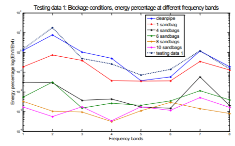
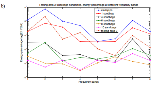
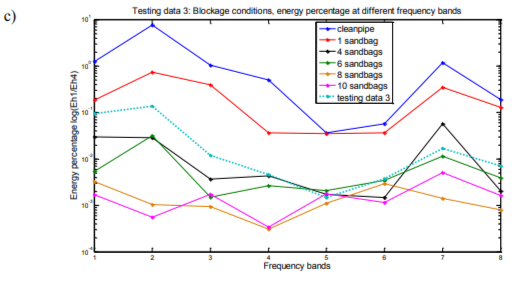
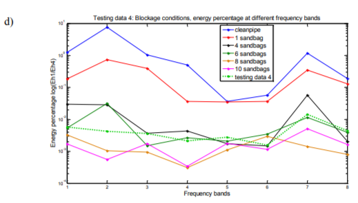
Figures of energy percentage against frequency bands of both testing data and training data support the results derived from K-nearest neighbors classification. Figure 5(a) shows the energy percentage against frequency bands of testing data 1 and 6 of training data sets, testing data 1 can be seen as closest to the training data of clean siphon condition which is class 1. It is the result similar to that obtained via the KNN classification method (see Table 6). Figure 5(b), (c) and (d) are testing data 2, 3 and 4 plotted in the same way with same training data sets as in Figure 5(a). All 4 figures illustrate the results consistent with those obtained via the KNN classification method.
а)
5. CONCLUSIONS
Discrete wavelet transform was used as a main signal processing method in reproducibility test, feature extraction and condition classification. Acoustic signals were decomposed into different frequency ranges up to 5512 Hz. The energy percentage and cross-correlation coefficients between individual data sets in each frequency band were calculated as characteristic features to describe the degree of similarity between these signals. The reproducibility analysis suggests that the data are reproducible if the condition does not change.
K-nearest neighbor algorithm was used as classification method to recognize the condition of the siphon. For this purpose the siphon was blocked with a controlled amount of sand. The results suggest that the acoustic technique and the adopted classification system are capable of discriminating different pipe conditions, but further refinements are needed to tune its sensitivity and improve its accuracy. Meanwhile, it also can be seen that the low frequency components of the signal appear to show more accurate results than their high frequency counterparts. Therefore, choosing frequency bands carefully helps to achieve better performance of the adopted classification method and it deserves a further investigation.
[1] This work was presented at the International Conference on Condition Monitoring and Machinery Failure Prevention Technologies in 2011. Published with permission of the British Institute of Non-Destructive Testing.
© The British Institute of Non-Destructive Testing, 2011.
Литература
- Grosse C. U., Finck F., "Improvements of AE technique using wavelet algorithms, coherence functions and automatic data analysis", Construction and Building Materials Vol 18, pp 203213,2004.
- Cohen L. "Time-frequency Analysis", Prentice-Hall, New York,1995.
- Debnath L, "Recent developments in the Wigner-Ville distribution and time-frequency signal analysis", PINSA, 68.A.No 1, pp 35-56, 2002.
- Michael Cowling R.S., "Comparison of techniques for environmental sound recognition", Pattern Recognition Letters, pp 2895-2907, 2003.
- Richard O., Duda P.E., "Pattern classification", John Wiley & Sons,Inc., New York, 2001.
- Singh B.N., Tiwari A.K., "Optimal selection of wavelet basis function applied to ECG signal denoising", Digital Signal Processing, Vol 16, pp 275-287, 2006.
- Strang G., "Wavelets and filter banks", Wellesley-Cambridge Press,Wellesley MA, USA, 1996.
- Hugo T., Grimmelius Meiler P.P., Maas H.L. and Bonnier B., "Three state-of-the-art methods for condition monitoring", IEEE Transactions on Industrial Electronics, pp 407-416, 1999.
Информация об авторах
Метрики
Просмотров
Всего: 839
В прошлом месяце: 2
В текущем месяце: 2
Скачиваний
Всего: 710
В прошлом месяце: 0
В текущем месяце: 0