Моделирование и анализ данных
2012. Том 2. № 1. С. 25–34
ISSN: 2219-3758 / 2311-9454 (online)
Novel probabilistic algorithms for dynamic monitoring of electrocardiogram waveforms
Аннотация
Novel algorithms for dynamic monitoring of electrocardiogram waveforms are presented. Their objective is to measure drug-induced changes in cardiac rhythm, principally by means of the QT-interval.
Общая информация
Ключевые слова: Electrocardiogram waveforms, Hidden Markov models
Рубрика издания: Научная жизнь
Тип материала: научная статья
Для цитаты: Strachan I. Novel probabilistic algorithms for dynamic monitoring of electrocardiogram waveforms // Моделирование и анализ данных. 2012. Том 2. № 1. С. 25–34.
Полный текст
1. INTRODUCTION
In this paper we present two novel algorithms for dynamic monitoring of electrocardiogram waveforms (ECG). The objective of the algorithms is to measure drug-induced changes in cardiac rhythm, principally by means of the QT-interval - the time between the onset of ventricular depolarisation and the end ventricular repolarisation. This is a recognised biomarker which may indicate increased risk of cardiac arrhythmia, which may arise if the action of a drug prolongs this interval.
Conventional analysis of the QT interval is performed on individual ECG beat waveforms by trained cardiologists, who perform mark-ups of the waveform on screen using digital callipers. Our techniques minimise the amount of work needed to be performed by exploiting an existing database of mark-ups as a training set for an automated method using hidden Markov models. Once an initial automated analysis is performed on a continuous recording which may over twenty-four hours consist of around 100,000 beats, a small set of less than 30 “template beats” are then generated for a Cardiologist to inspect and mark-up. These template mark-ups may then be used to perform a re-annotation of the recording.
The rest of this paper is arranged as follows:
- In section 2 we give a brief description of the clinical background to the application
- In section 3 we describe the hidden Markov model implementation of the automated ECG analysis
- In section 4 we describe how template beats summarising a whole ECG recording are generated and used to provide an additional analysis.
2. CLINICAL BACKGROUND
The electrocardiographic QT interval is an important measurement because when abnormally prolonged, it is a warning sign of both cardiac and arrhythmic death [1]. In addition, most regulatory authorities require an assessment of the effect of new drugs upon the QT interval for their approval and appropriate labelling [2]. This assessment, known as a Thorough QT Study is performed on a set of healthy normal subjects, who are given doses of placebo, the drug under study, and a control drug with a known QT prolongation effect. Typically, 10-second ECG recordings are made at specified timepoints after dosage, which can be analysed manually. However, the QT interval itself is highly variable from beat to beat (it can vary by as much as 10-15 ms between beats, where a systematic prolongation of 15 ms is likely to be of regulatory interest. This motivates the use of continuous ECG recordings using an ambulatory Holter ECG recording device. This, coupled with an automated measurement system, allows the measurement of an enormous number of ECG beats, whose subsequent averaging over a time period is likely to give a truer picture than an intermittent 10 second recording.
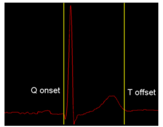
Figure 1. QT interval marked up on a standard beat.
Figure 1 shows a standard ECG beat, with yellow markers denoting the QT interval; the three turning points following the first yellow marker are known as the QRS complex, and correspond to ventricular depolarisation, when blood is pumped out from the ventricles. The smaller peak before the second yellow marker is known as the T-wave, and corresponds to ventricular repolarisation, when the ventricle relaxes in preparation for the next beat.
The motivation for measurement of the QT interval is that certain drugs are known to affect the cardiac repolarisation cycle and cause a prolongation of the interval. This can increase the risk of a particular cardiac arrhythmia, known as Torsades de Pointes (TdP), which, though not fatal in itself, can easily degenerate into ventricular fibrillation, which is fatal. The waveform of TdP is shown in Figure 2.
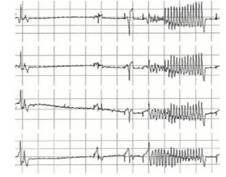
Figure 2. Torsades de Pointes.
3. AUTOMATED QT ANALYSIS BY HIDDEN MARKOV MODEL
Our algorithm for automated analysis of the ECG waveform and measurement of the QT interval utilises a hidden Markov model [3] (HMM), based on work by Hughes [4]. The HMM is used to segment up the waveform into different regions, corresponding to different states of the model. This is analogous to the use of HMMs in speech recognition, where the different states of the model correspond to different phonemes [3].
One possible configuration of the state transition diagram for an HMM-based ECG analyzer is shown in
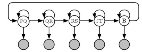
Figure 3. State transition diagram for HMM-based ECG analyzer.
Here, the states are labeled according to the different peaks within the ECG waveform; the P wave corresponding to the atrial depolarization, the Q,R, and S peaks corresponding to ventricular depolarisation, and the T wave corresponding to ventricular depolarization. The point at the end of the S wave (end of the QRS complex) is termed the J-point by cardiologists. The “B” state corresponds to the isoelectric baseline that occurs between beats. This hidden Markov model can be used to automate the process of placing mark-ups on an ECG wave, by using the Viterbi Algorithm, which is a method based on dynamic program whereby the optimal sequence of states in a hidden Markov model can be computed [5]. Once the optimal sequence of states is computed, this can be used to place mark-up points corresponding to the state transitions from one state to the next (the horizontal arrows in the state diagram). In this case, the beginning of the QT interval would correspond to the transition between the PQ state and the QR state, and the end of the QT interval would correspond to the transition between the JT state and the B state.
The emission probabilities (probabilities of the individual states at each time point) are computed from feature vectors derived from the Undecimated Wavelet Transform (UWT) of the signal[6].
The training of the HMM differs from the traditional approach using the Baum-Welch reestimation algorithm [3] in that in our case, a database of 18,000 ECG waveforms were used which already had the state transition positions provided as mark-ups by Cardiologists. Hence, the positions of the state transitions are known beforehand, and the matrix of transition probabilities can be computed by counting the durations within each state.
The emission probabilities are formed as Gaussian Mixture Models, whose parameters are learnt by an Expectation-Maximization algorithm [7].
The result of running the Viterbi algorithm on an HMM trained in this manner is shown in Figure 4, where the state labels are shown on the X-axis, and the optimal sequence of states is shown in light blue. The transition from the state PR to the state QRS is the beginning of the QT interval, and from Tw to B2 is the end of the T wave and the end of the QT interval. In this model, the states were defined somewhat differently than in the state transition diagram of Figure 3, that: the interval from the start of the P-wave to the start of the Q wave is traditionally called the PR-interval by cardiologists, the QR and RS states are merged into one state, and the T-wave has been divided into two states Tb (baseline to start of T-wave) and Tw (T-wave itself). The onset of the T-wave was deduced by heuristic methods from the database of ECGs used as an interval before the peak of the T-wave equal to the interval between that peak and the marked end of the T-wave. It does not matter that this is not a precise method, because the objective is simply to split it into two states with no particular need to have an accurately determined transition point.
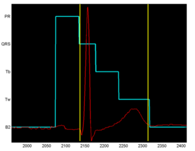
Figure 4. Output from Viterbi algorithm on the trained HMM.
An important advantage of our algorithm over existing automated techniques is that it is a probabilistic technique and can therefore give a principled estimate of the confidence of measurement. Existing techniques for estimation of the end of the T-wave, for example, rely on heuristic measurements of the gradient of the down slope of the T-wave and the baseline. These do not give a probability, and hence will always output an answer even if the waveform is corrupted by noise. By contrast, our algorithm will produce a low value of confidence if the waveform is corrupted, and by application of a confidence threshold, we are able to exclude corrupted beats from the analysis. This is illustrated in Figure 5, which shows the results of using the algorithm to analyse a 24 hour continuous ECG recording of a patient on the beta-blocker drug Sotalol, in a study by Sarapa et al [8]. In this recording, 76954 beats were analysed in total. In the figure, we have plotted the 30-second averages of the QT interval in milliseconds as a function of the time after dosage. We have plotted in red the points where the average level of confidence over the 30 seconds was below a threshold. As can be seen, the low confidence beats tend to have been evaluated as a very short QT interval - in the case of this particular drug because one of the effects, as well as the lengthening of the QT interval (by around 90 ms in this example) is a flattening of the T-wave, which sometimes makes it difficult to locate the end.
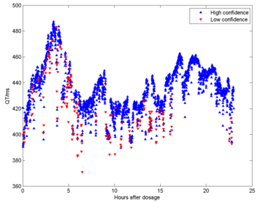
Figure 5. 24 hour QT analysis from a patient on Sotalol.
4. SEMI-AUTOMATED QT ANALYSIS BY SUBJECT-SPECIFIC TEMPLATES
While the confidence measure produced by the automated QT algorithm is a form of self-validation, it is also thought appropriate by the regulatory authorities to have human involvement in the review of the results produced. To this end, the second algorithm presented here utilises results produced by the automated algorithm to produce a set of “representative beats” that are then analysed, and if necessary re-annotated by a qualified cardiologist. The resultant mark-ups can then be used to re-apply measurements of the QT interval in a second phase, where the particular preferences for placement of the end of the T-wave of the Cardiologist in charge of the study are taken into account. The steps towards generating template beats are as follows:
- Perform a clustering algorithm, such as k-means on feature vectors extracted from the high- confidence beats from the automated analysis.
- For each cluster, form a template beat as an average of the beats that were associated with that cluster.
The key challenge here is to form an appropriate feature vector upon which to base the cluster. One of the most prominent effects of drugs on the ECG waveform is not only the change in QT interval, but also the change in the shape (morphology) of the T-wave. One method would be to extract feature vectors of fixed length from the T-wave and use this as the basis of the clustering in Step i. above. However, this neglects the fact that QRS morphology can also change independently from the T-wave morphology. In order to overcome this, we have adopted a novel clustering algorithm based around the Sammon Map, which is a form of multidimensional scaling that produces a low-dimensional visualisation that attempts to preserve Euclidean distances in feature space, according to the Sammon “Stress Metric”:
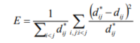
Where  is the distance metric between Beat i and Beat j and
  is the Euclidean distance be- ij ij
tween the two points representing each beat in the visualisation space.
In order to do this, we need to define a distance measure between two beats; this could be performed by feature extraction, but we have here adopted a method that relates directly to how the templates are generated; by normalising two beats to the same length using Dynamic Time Warping, another technique used commonly in speech recognition[9]. This process is illustrated schematically in Figure 6. The procedure, which is based on dynamic programming, involves a non-linear stretching of the time axes of two signals (in this case the two beats to be compared), in order to minimise the summed square differences between the two signals. Once this has been performed, a root mean square distance can be computed for the two signals, which corresponds to a normalised Euclidean distance (per time sample).
Hence we could perform a Sammon projection on a high-confidence subset of the beats in a recording, and then perform the clustering in the visualisation space, in order to select the candidate beats for each template.
However, one significant challenge remains to be overcome to make this method feasible. The biggest disadvantage of the Sammon map is that, as can be seen from equation (1), the computational complexity of the algorithm scales as the square of N, the number of data points.
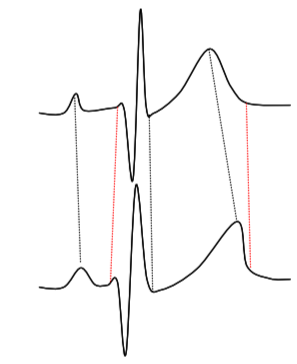
Figure 6. Schematic illustration of Dynamic Time Warping.
This would render the method infeasible, especially since the distance calculation we need to perform for ![]() is not a simple Euclidean distance between two vectors, but is instead a Dynamic Time Warp operation, which is computationally considerably more expensive.
is not a simple Euclidean distance between two vectors, but is instead a Dynamic Time Warp operation, which is computationally considerably more expensive.
So instead, we have introduced a modification of the Sammon algorithm [10], that greatly reduces the computational load. This is achieved by noting that the Sammon Stress objective function is simply a sum of terms dependent on pairs (i,j) of vectors. In practice, it has been found that one can leave out many of the distance pair calculations, and still produce a mapping that is very similar to the Sammon Map. Thus we define a sparse subset S of the set of interpoint distances, by choosing, for each point, a randomly selected subset of the other points. In practice this can be a small fraction of the available data. We term the new metric SASS (Sparse Approximated Sammon Stress), which is formally defined in terms of the sparse subset S as follows:
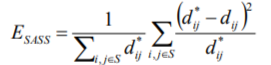
By choosing, for example 5000 high confidence beats from a recording, and having each beat compared randomly with around 100 others, it is possible to pre-compute the distance matrix  in a few minutes on a standard PC. The pre-computed distance matrix is then used as an input to the optimisation algorithm, to produce a 2-Dimensional map that can then be clustered, using k-means clustering. For each cluster so formed, we then form a template by again using Dynamic Time Warping, choosing the most typical beat (closest to the cluster centre) as the starter beat, and then warping all the other beats in the cluster onto that beat.
The results of this are summarised in Figure 7 for a subject on Placebo in the Sarapa et al So- talol study [8]. The left hand plot in the figure shows the visualisation of 5000 beats that were selected from the automated analysis. Each blue circle represents a single beat, and the distances between points on the graph are optimised to approximate as closely as possible the pairwise distances from the Dynamic Time Warping procedure between the corresponding beats. The red dots on the graph are result of performing k-Means clustering on the visualisation points, in this case producing 10 cluster centres,
giving rise to 10 templates to summarise the recording. The green squares are the 453 beats associated with one particular cluster. The resultant template is shown in the right hand plot, with the template itself shown in red, and the corresponding family of beats used to generate the template shown in light blue. It should be noted that there is an acceptance criterion (based on the Dynamic Time Warp distance) associated with the procedure, and in this case 339 of the beats have been accepted. The blue vertical lines represent an initial estimate of the QT interval mark-ups, which will be subsequently examined by a cardiologist and if necessary adjusted.
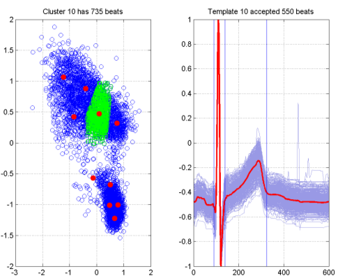
Figure 7. Template generation via SASS.
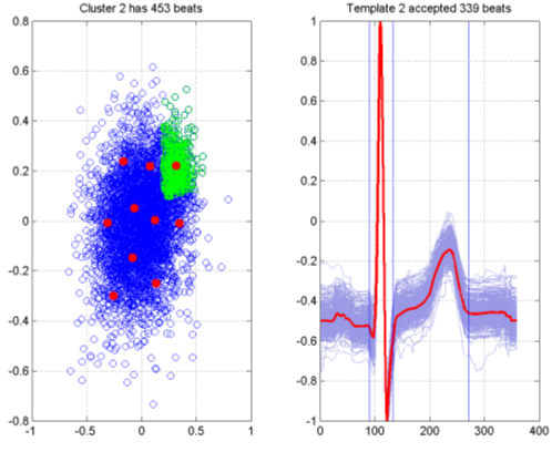
Figure 8. Template Generation from SASS - Sotalol dosage.
Figure 8 shows the corresponding plot for the same patient when on a dosage of Sotalol, as opposed to a placebo. The visualization has the added benefit of showing a marked change in the variability of the beat morphology (this can be seen by comparing the scale of the axes in the two figures. The effect of the drug has been to produce a much larger and more diffuse cluster of beats, shown above the main cluster, which is densely packed. One of the templates is shown in the right hand plot, showing a marked difference in the T-wave morphology as a result of the drug effect.
Following the generation of templates and adjustment of markups by a Cardiologist, a recording can be re-analysed using the Cardiologist markups of the templates as a basis. This is performed by a reverse Dynamic Time Warp process, where the template is warped back onto the beat and the mapped positions of the beginning and end of the QT interval are computed. This is termed the “refined” analysis - as the measurement of each beat is based on a subject-specific set of mark-ups from a single Cardiologist, as opposed to a subject-generic analysis based on mark-ups from many Cardiologists, which was the basis of the training data.
Typical results from this are seen in Figure 9, for a patient on Placebo. It is noticeable from this that the scatter of points from beat to beat for the QT interval is lower for the refined analysis than it is for the automated analysis; more detail can be seen, and in one case, it has been possible to restore some low confidence beats that were omitted from the initial automated analysis.
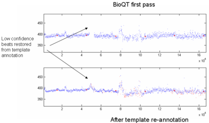
Figure 9. Refined data analysis compared with automated algorithm.
[1] This work was presented at the International Conference on Condition Monitoring and Machinery Failure Prevention Technologies in 2009. Published with permission of the British Institute of Non-Destructive Testing.
© The British Institute of Non-Destructive Testing, 2009.
Литература
- Kass R. S. and Moss A. J., “Long QT syndrome: novel insights into the mechanisms of cardiac arrhythmias”, J Clin Invest, 2003, Vol 112, No 6, pp 810–815.
- “International Conference on Harmonisation. Guidance on E14 clinical evaluation of QT/QTc interval prolongation and proarrhythmic potential for non-antiarrhythmic drugs; availability”, Notice Fed Regist, 2005, Vol 70, No 202, pp 61134-61135.
- Rabiner L. R., “A tutorial on hidden Markov models and selected applications in speech recognition”, Proceedings of the IEEE, 1989, Vol 77, No 2, pp 257–286.
- Hughes N. P., “Probabilistic models for automated ECG interval analysis”, DPhil thesis, University of Oxford, 2006.
- Andrew J. Viterbi, “Error bounds for convolutional codes and an asymptotically optimum decoding algorithm”, IEEE Transactions on Information Theory, Vol 13, No 2, pp 260–269, April 1967.
- Shensa M.J., “The discrete wavelet transform: wedding the a trous and Mallat algorithms”, IEEE Trans. Signal Processing, 1992, Vol 40, pp 2464–2482.
- Hughes N.P. and Tarassenko L., “Probabilistic models for automated ECG interval analysis”, Submitted to: IEEE Trans. Biomedical Engineering.
- Sarapa N., Morganroth J., Couderc J.P. et al, “Electrocardiographic identification of drug-induced QT prolongation: Assessment by different recording and measurement methods”, A.N.E., 2004, Vol 9, No 1, pp 48–57.
- Holmes J. R. and Holmes W. Speech Synthesis and Recognition (2nd Edition), Taylor and Francis, 2001.
- Wong D., Strachan I., Tarassenko L., “Visualisation of high-dimensional data for very large data sets”, Proc. 25th International Conference on Machine Learning – Workshop on Machine Learning for Health Care Applications (Helsinki, Finland, 2008).
Информация об авторах
Метрики
Просмотров
Всего: 813
В прошлом месяце: 3
В текущем месяце: 1
Скачиваний
Всего: 544
В прошлом месяце: 0
В текущем месяце: 1