Моделирование и анализ данных
2012. Том 2. № 1. С. 51–58
ISSN: 2219-3758 / 2311-9454 (online)
Hidden Markov models in task of condition monitoring
Аннотация
This paper describes hidden Markov models use in technical objects condition monitoring. A hidden Markov model is a statistical model in which it is assumed that a system is Markov process with unknown parame¬ters. Based on observations generated by the system, model parameters are extracted. Models described by these parameters are used for further analysis and prediction studies. The paper discusses relationships and differences between a visible Markov model and its hidden counterpart. In considered task hidden Markov models are used to detect changes in the technical state of examined object. The main problem of method developed is to elaborate method which will be able to detect significant changes in a system observation vector and ascribe a given observation to the present technical state. An example of using hidden Markov models for rolling bearings is presented.
Общая информация
Ключевые слова: Hidden Markov models, condition monitoring, vibro-acoustic signals, signal symbolization, bearings
Рубрика издания: Научная жизнь
Тип материала: научная статья
Для цитаты: Gałęzia A., Radkowski S. Hidden Markov models in task of condition monitoring // Моделирование и анализ данных. 2012. Том 2. № 1. С. 51–58.
Полный текст
1. INTRODUCTION
Modern research is often aimed at building such a diagnostic system which will allow to determine the technical state of tested object. Correct and certain determination of technical state is important in condition monitoring and makes it possible to determine future operating strategies for minimizing operating costs and failure hazards. Change of technical state is usually connected with changes in the object kinematics, development of failures, changes in cooperated kinematics pairs.
The most often occurring machine components are bearings, gearboxes, shafts and couplings. Their failures and disturbances in kinematics are often examined to develop new diagnostic methods, to acquire knowledge for expert systems and examine condition monitoring techniques. The other options to assess the technical state or maintenance affects provides the hazard function. Markov models can be used to represent certain degradation processes for many elements of power transmission unit, especially when the likelihood of being in any particular state in the next time interval depends only on the present state. In this case measurement data are used to estimate the probability of transition from one state to the other with assumption that the deterioration level k can be reached only from deterioration level k-1.
Information about technical state of machine can be obtained from signals generated by the machine examined. The signals can be vibro-acoustic, electrical (in case of electrical engines), and many others. Usually vibro-acoustic signals generated by a machine component are disturbed by other sources of signals and noise. Extraction of diagnostically useful information from signals can be very hard and often needs complicated signal processing methods.
The paper presents idea of usage of symbolization of time series of diagnostic signals, visible and hidden Markov models in task of condition monitoring. Also, further research which will be carried out on a laboratory stand is described. Firstly, the general methodology of stage classification consists in creating a symbolic signature which is characteristic for a given signal, and then using Markov models to infer which, most probably, model of anomaly resulted in the observed signal and which technical stage this signal corresponds to.
2. SYMBOLIZATION OF DIAGNOSTIC SIGNAL TIME SERIES
The idea of diagnostic signal symbolization is based on research works of A. Ray, C.S. Daw and others [1, 2]. Also, earlier research works of the authors [3] have contributed to the present paper. In general, the idea of time series symbolization can be described as transformation of raw time domain signal into a set of symbols. There are two basic parameters of symbolization process - symbolization frequency and quantization parameter - which have influenced symbolization. The former defines how often a sample of original signal is selected and based on quantization parameter, or value of sample a given symbol is chosen (Figure 1).
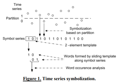
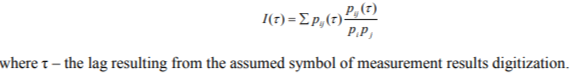
Quantization parameter is related with partition chosen on raw data and the alphabet. The latter contains all available symbols which can be ascribed to samples of signal. Symbolization process results in a symbol series which, assumingly, provides equivalent diagnostic information as a raw time signal. To verify this assumption, correct value parameters must be chosen. However, there is no one correct method of selecting symbolization parameters for the raw signal symbolization. In literature, one can find description of several methods used for calculation of symbolization frequency and quantization such as mutual information function [3]: where т - the lag resulting from the assumed symbol of measurement results digitization.
Time signal symbolization can be treated as transformation of raw signal into new space. It should be pointed out that it is possible to use various signal analysis techniques for symbolic series to extract some additional diagnostic information. From symbol series, using a given length template sliding along symbol series, a set of the so called words is created. Words are sets of symbols from symbol series. They can overlap with a given number of elements. A set of words allows to create a word occurrence statistics, such as a histogram, and later to make a suitable word occurrence analysis. Thus, for a given signal a distribution of amounts of words is created that can be treated as a characteristic signature of signal. Another signal signature can be a transition matrix, which contains distribution probability of transitions from one word to another. Example of transition matrix of 4 words is presented in Table 1, where Pij is a transition probability from Word i to Word j.
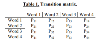
Comparison of histograms and transition matrixes for different signals can be made only for symbolic series created with same parameters. Example of differences between transition matrixes of two signals can be found in [4].
Authors propose a different view of symbolic transformation: a given signal can be transformed into symbolic signature based on values of raw time signal diagnostic parameters. The basic assumption is that a given signal can be connected with a technical state. To explain the idea of approach suggested, the following simple example will be used: a set of diagnostic parameters will be calculated from different signals, based on their values different signatures typical of the signal, will be created. For convenience 4 basic signals were created, a set of two simple diagnostic parameters, RMS and PEAK, was chosen and binary symbolic alphabet was defined. Each of basic signals (Figure 2) differed with values of RMS and PEAK parameters.
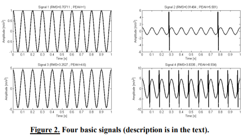
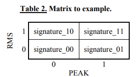
From each signal a value of RMS and PEAK was calculated. Based on proposed parameter thresholds a set of diagnostic parameters [RMS, PEAK] was transformed into a symbolic set [RMS_symbol, PEAK_symbol]. It was assumed that if RMS value was lower than 1, then symbol 0 was described as RMS_symbol in a symbolic set, else symbol 1 was ascribed. If PEAK value was lower than 5, then symbol 0 was described as PEAK_symbol in a symbolic set, else symbol 1 was ascribed. Thus, each signal has received its own symbolic signature, i.e. [0, 0], [0, 1], [1, 0] or [1, 1].
It is possible to define bigger sets of reconsidered diagnostic parameters by simply adding the ones which will make symbolic signature more sensitive for signal parameter change. In addition, a symbolic alphabet can be increased giving higher sensitivity of a symbolic parameter to changes of its signal counterpart. This procedure can be treated as diagnostic parameter quantization. As a result, a matrix presented in Table 2 can be created. This matrix informs which signature from all possible possesses the examined signal.
3. VISIBLE AND HIDDEN MARKOV MODELS
A hidden Markov model (HMM) is a two-layer statistical process in which, first, an underlying process is not observable (it is hidden) and can be observed only due to the second stochastic process which produces visible observations. They are probabilistic functions of the states. HMM is fully described by a set of 5 parameters (S, O, A, B, П), where:
S is a finite set of N-states, O is a finite set of M-possible symbols, A is a set of state-transition probabilities, B refers to observation probabilities, П means initial state probabilities. HMM with its parameters is marked as X=[A, B, П]. Details related with creation, a training process and other HMM features can be found in [5, 6].
In the abstract the term “visible Markov model” was used by the authors, who believe that visible Markov model can be treated as a special HMM case. Similarly, as in case of HMM, visible Markov model is based on the same 5 parameters (S, O, A, B, П). However, in case of visible model it is assumed that matrix B uniquely connects the state with observation, which is no longer the state probabilistic function, or more exactly the probability of emitting characteristic observation ok by actual state qt P{ok/qt = S■} = 1. With this definition visible Markov model seems to be very similar to Markov chain. However, in Markov chain a sequence of states is observed, there is no concept of observation as a second overlying process. Markov chain is fully described by (S, A, П). By this term the authors would like to draw attention to a close relationship between visible and hidden Markov models. The basic difference between visible Markov model and its hidden counterpart is connected with matrix B and makes that in terms of flexibility visible model has less degree of freedom. A training process based on Baum-Welch algorithm for visible Markov model changes A and П parameters but no B. Visible Markov models can be used in a preliminary test of state classification algorithm as a first step before HMM application. For a real object state classification HMMs must be used due to existence of noise and other random disturbances which influence diagnostic signal and might give different observations for the same technical state. Classification system must be flexible and must be able to accept reasonable differences. HMM training procedure is based on learning data, which determine the quality of trained model. To choose these data is difficult and requires much experience. It is also important in preliminary choice of HMM parameters from which Baum-Welch algorithm will start training. A problem of this training algorithm is that it might reach local maximum. Training seems to be started several times, with different starting parameters each time.
For failures and disturbances analyzed, different models are created. The signal analyzed is compared with models and likelihood parameter is calculated for each model. The one with the highest likelihood marks the most probable state.
4. CLASSIFICATION SYSTEM EXAMPLE
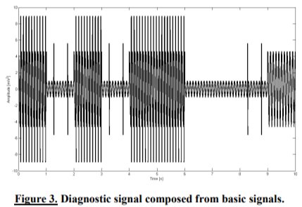
To verify the idea of symbolization and hidden Markov model application in condition monitoring, a preliminary research was made. Four diagnostic signals were created, each of them composed from four basic signals presented in Figure 2, and supposed to characterize different states. Figure 3 presents example of such signal.
Each signal was subjected to the same symbolization procedure. Firstly, a signal was divided into parts of same length, 1000 samples. From the signal 100 parts were obtained. For each part a diagnostic vector consisting of RMS and PEAK values was calculated. As a result, the same number of succeeding diagnostic vectors as a number of parts of original signal was obtained. Then, depending on parameter threshold values an adequate symbol from the alphabet was ascribed and a symbolic vector was created. The resulting set of symbolic vectors was submitted to the occurrence analysis - an amount of different vectors for different signals was calculated and compared. It was assumed that change in occurrence matrix is due to change of state (Figure 4).
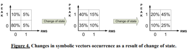
Observation of changes in occurrence matrix informs about change of state, simultaneously the control of exact values of diagnostic parameter informs about direction of changes (Figure 5).
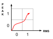
Figure 5. Changes in symbolic vector occurrence as a result of change of state.
Deeper layer analysis can be carried out to detect the process causing these changes, whether it is, for example, amplitude or frequency modulation or square element appearance in signal. Such analysis is also based on the symbolization idea discussed above. E.g., for amplitude modulation and binary partition, a ratio of minimum amplitude to maximum amplitude is calculated. Defying that if this ratio is e.g. lower than 0.9, then symbol 1 is assigned to a symbolic vector (else 0), a new symbolic vector for a new parameter set is created. Thus, it is possible to make simple analysis of signal structure.
To use hidden Markov models in task of state classification, a set of states and observations must be defined. The latter might include specific signal signatures like symbolic vector occurrence matrix.
Working on this subject the authors used open to public MATLAB procedures for HMM calculations [7, 8]. From many available toolboxes they seem to be well described and prepared. Also last versions of MATLAB Statistics Toolbox contain functions useful for work with HMM.
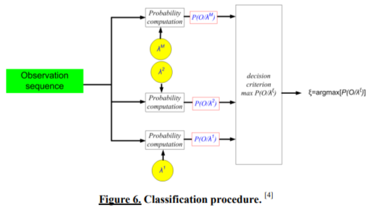
During research appropriate models were created for each of 4 technical states. Observations used in models were symbolic vector occurrence matrices. For each model a training process was carried out for typical data characteristic feature for a given state. The models prepared were saved in file data base. Then, a testing signal consisted of basic signals was also generated. It was symbolized with same procedure as signals used to create models. To carry out a classification procedure, probability, that the analysed observation was generated by different hidden Markov models, was calculated (Figure 6). Basing on value of likelihood classification is carried out.
For analysed case, such way created system, worked fast and was able, for most cases, to give correct answer of classification.
For the analysed case, the system created consisted of basic signals, worked fast, and, for most cases, was able to give correct answer of classification.
5. FUTURE WORK AND CONCLUSIONS
In the nearest future, additional work will be carried out for developing the system, vectors of diagnostic parameters and symbolization procedure. The test stand composed of two electric engines (motor and dynamometer), one stage gearbox, a shaft with unbalance disk, two bearings, and couplings is being put in motion (Figure 7). Construction on allows for easy change of bearings and realization of additional failures and errors.
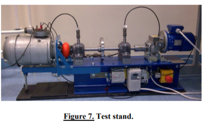
To verify the proposed methodology, the diagnostic signal will be recorded from the test stand. During measurement campaign signals will be recorded for different motor rotational speeds and different loads generated by dynamometer. Also bearings with different failures will be tested. The authors mainly aim to detect the early stage of failure. Test stand allows for implementation of different errors such as unbalance, bearing support clearance, different types of misalignment.
Based on the simulations already available, the proposed method of object technical state classification seems to be promising. Further research will reveal advantages and disadvantages of symbolic state classification using hidden Markov models.
Acknowledgements
This work has been supported by the European Union in the framework of European Social Fund through the Warsaw University of Technology Development Programme.
[I] This work was presented at the International Conference on Condition Monitoring and Machinery Failure Prevention Technologies in 2009. Published with permission of the British Institute of NonDestructive Testing.
© The British Institute of Non-Destructive Testing, 2009.
Литература
- Daw C.S., Finney C.E.A., Tracy E.R., “A review of symbolic analysis of experimental data”, http://www-chaos.engr.utk.edu/pap/crg-rsi2002.pdf.
- Ray A., “Symbolic dynamic analysis of complex systems for anomaly detection”, Signal Processing, Vol 84, 2004, pp 1115-1130.
- Galezia A., Radkowski S., “Problem of proper choice of discretization and quantization in symbolic transformation of signals”, Proceedings of the Third WCEAM-IMS, pp 509-514, 2008.
- Galezia A., Radkowski S., “Usage of symbolic analysis in condition monitoring”, Proceedings of the fifth International conference on Condition Monitoring and Machinery Failure Prevention Technologies, UK, 2008.
- Rabiner L.R., “A tutorial on HMM and selected applications in speech recognition”, Proceedings of the IEEE, Vol 77, No 2, pp 257-286, February 1989.
- Ibe O.C., “Markov processes for stochastic modelling”, Elsevier Academic Press, Oxford, UK, 2008.
- http://www.cs.ubc.ca/~murphyk/Software/HMM/hmm_usage.html.
- http://www.igi.tugraz.at/lehre/CI/tutorials/HMM.zip.
Информация об авторах
Метрики
Просмотров
Всего: 919
В прошлом месяце: 2
В текущем месяце: 1
Скачиваний
Всего: 403
В прошлом месяце: 0
В текущем месяце: 0