Tensor Network Model of Logistics System

The goal is to create a network model of logistics that ensures the distribution of product flows from producers to consumers in conditions of growing volumes of information, changing economic ties. To create a model, a tensor method of calculating processes is used when changing the structure of network models of technical and economic systems, including decomposition and calculation in parts. The network is considered as a tensor, the projections of which are various connections of branches. The coordinates in the network space are closed and open paths. When changing the network structure, a new solution is obtained using a path transformation matrix. As a result, for the first time, a network model of logistics was created with branches of producers, consumers (determine the basis of open paths) and routes (determine the basis of closed paths). The resistances of the branches set the tariffs for the storage and transportation of products. The product flows of producers and consumers are set by voltage sources that create part of the distribution of flows along routes. To supplement up to full product flows, voltage sources are introduced in the branches of the routes, which give additional currents. For routes in excess of the number of open paths, the values of the complement currents should be selected. The sum of currents from all sources gives the values of product flows from suppliers to consumers, solving the logistics task. The network model is used to calculate product flows along routes without iterations, the cost of transportation, as well as to transform the solution when routes, tariffs, supply and demand change, using algorithms of the tensor method of dual networks.

Introduction

The task of logistics is to transport product flows along routes that connect producers and consumers. Routes are characterized by the cost of transportation (tariffs), length and throughput. The logistics system creates networks for the movement of product flows in the conditions of growing volumes of information, changes in technologies, routes, tariffs, supply and demand. Calculating the distribution of product flows in logistics systems, as well as their changes, requires performing large amounts of calculations that are necessary for supply chain management.

The purpose of the study is to create a network model of logistics that ensures the distribution of product flows from producers to consumers, allows you to use ready-made solutions to obtain new solutions in conditions of change.

The distribution of product flows is an important logistics task, to which many studies are devoted. In a linear programming transport problem, products are transported along routes or stored in warehouses. The cost of transportation and storage in warehouses of goods is set by a combined matrix. It is necessary to determine the routes that provide transportation in the shortest time, or at the lowest cost. It is assumed that the sum of supplies is equal to the sum of demand.

Various methods of solving the transport problem are known. For example, the northwest angle method, the Vogel approximation method, the differential rent method, the potential method, which use variants of the simplex method. First, the flows are distributed between the destinations and receive a reference plan. In subsequent iterations, the optimal plan is determined by improving the current reference plan. These methods use iterations and do not provide a transition from existing solutions to solutions of the problem for new conditions, for example, route changes. The well-known Ford-Fulkerson algorithm of iterative search for the maximum flow in the transport network converges for entire throughput capacities, but even for them it can work for a very long time.

The topological model in the form of an equivalent electrical circuit for the transport problem was developed by G. Kron [1]. The model is designed to solve the linear programming problem in parts, and optimize the cost of transportation. The model turned out to be difficult to apply. G. Kron believed that the simplex method is simpler and more efficient, but the physical interpretation of the network model will allow the calculation to be applied in parts.

The purpose of this study is to create a network model that distributes product flows in two calculation stages without iterations and provides a solution change when routes, tariffs, supply and demand change.

It was possible to establish analogies and represent the flows of products in the logistics system by currents in the electrical circuit; where tariffs are set by resistances, and voltages give the cost of transportation. The solution has the properties of optimality, since the electrical circuit, connecting the processes and structure by the laws of Ohm and Kirchhoff, obeys the principle of least action.

For practice, it is important that the network model allows you to apply the tensor method of calculating networks when changing the structure, including decomposition and calculation by parts of complex logistics systems. The tensor method of dual networks [2] provides calculation without iterations due to the duality invariant found by the author. This method is relevant for the decomposition and application of parallel computing in conditions of growing volumes of information in logistics and supply chain management systems.

Literature review

Works on the distribution and transportation of product flows in the logistics system is being carried out in the direction of analyzing the growing volumes of information and applying logistics methods in other subject areas.

The first network model of the transport problem in the form of an electric circuit was developed, as noted, by G. Kron [1]. There are six types of quantities in the circuit: impedances and conductivities, contour voltage sources and response currents, nodal current sources and voltage responses. There are three types of values in the transport system: the quantity of goods, the cost of transportation and the cost of storage. Although Kron believed that tariffs should represent impedances, however, he then believed these values to be equal to units. In this case, the current and voltage in each branch are numerically equal. The costs of transportation and storage of product flows at the inlet and outlet were considered by Kron as voltage sources.

Kron presented the objective function for route selection as minimizing power, however, the voltage refers to the circuit network, and the current refers to the node network. The network model implements the simplex method of linear programming problems, which allows you to solve the problem in parts. Input and output streams are considered as current sources. The product flows correspond to the sum of nodal and contour currents, which remain constant in each branch. Changes in the connection of branches change the number of closed and open paths, while nodal and contour currents change.

Tensor network analysis is used to analyze transport systems in a number of works for engineering and economic analysis [5], optimization of the airline network [12], engineering calculations [13], damage analysis [14], and traffic flows [15, 16, 18]. Discrete tensor analysis is used for modeling on railway transport [20], for calculating a tensor network model based on the simplex Danzig method [22]; as well as in a traffic distribution model in a multi-level info communication network [25]. The search for balance in large transport networks using direct-dual accelerated methods and tensor optimization methods with auxiliary one-dimensional optimization is presented in [23-24]. The model of functional and structural reliability of the supply chain in logistics and supply chain management is considered in [26].

In this study, a tensor method of calculating processes when changing the structure of network models of technical and economic systems is used to create a model. The generalized system is considered as a tensor, the projections of which are systems of various subject areas. The  Diacoptics [1, 10, 13] presents network models of Maxwell, Schrodinger equations, nuclear reactor, building structures, electric machines, turbine blades, etc. The tensor method of dual networks [2, 3, 4] was the development of Kron's work based on the duality invariant (the law of conservation of energy flow) [6, 8]. The author created network models of intersectoral balance [2, 3], banks [3], security systems of oil refining facilities [21], placement of gas detectors for fire detection [27], shaft ventilation, etc.

The network model of the logistics system [18, 19] was the development of the tensor method application in a new subject area.

Tensor method of network calculation

To create a network model of the logistics system, the tensor method of dual networks developed by the author is used [3, 6, 8, 9]. The network consists of branches connected by a structure of links. The network is considered as a tensor, the projections of which into coordinate systems are various structures, branch connection schemes.

The coordinates in the network space are closed and open paths that make up orthogonal subspaces. A path is a line running along the branches, may or may not coincide with them in the direction. Paths may vary in the composition of the elements through which they pass, in orientation, and may close or open. Changing the structure of the system consists in changing the boundaries, connecting or disconnecting elements, for example, branches of the network. At the same time, the number of basic closed and open paths changes, which changes the dimension of their space, the path transformation matrices become rectangular; that is, they do not have inverses.

In a dual network, closed paths correspond to open paths, and vice versa, and connections correspond to disconnections, and vice versa. The sum of the dimensions of the spaces of basic closed and open paths in two networks is constant. The duality invariant is expressed by the constancy of the sum of metric tensors of two dual networks when the structure changes. This makes it possible to use networks to model systems of different subject areas. The duality invariant corresponds to the constancy of the sum of powers in two electric circuits with a dual structure when the connection of branches changes. This is how the law of conservation of energy flow manifests itself.

The simplest coordinate system is a network of separate branches, in which paths pass through their branches. Processes take place in the network as responses to the applied influences. The transition to a connected contour network is carried out using a path transformation matrix C, consisting of a submatrix of the transformation of closed paths ^mC and a submatrix of the transformation of open paths ^jC. The transition to a connected node network is carried out by a matrix of transformation of paths of mutual basis A = C^-1_t; consisting of a submatrix of transformation of closed paths ^mA and a submatrix of transformation of open paths ^jA.       

In a dual network, the matrices С и А are swapped [2, 3, 8, 9].

An abstract network is clearly represented by an electrical circuit in which the processes are described by Ohm's law, e_a = Z_ab i^b, both in the simplest network and in a connected network. The structure is described by Kirchhoff's laws: the sum of the currents in the nodes is equal to zero and the sum of the voltages in the contour is equal to zero.

The voltage sources in branches, e₀ are internal influences. Responses, currents arise in branches, the basis is closed paths, contours. The calculation is carried out as a transformation of the solution of the simplest network into a solution of a connected contour network using the path transformation matrix ^mC [3, 4].

i_с = ^mC_t i` = ^mC_t (^mC Z ^mC_t)^{-1 m}C e₀ = Y_c e₀                                             (1) 

where i_c is the measurable currents in the branches of the network, i` is the currents in the contours of the basis, e₀ is the specified voltage sources, Z is the impedance matrix of the simplest network, Y_c is the solution matrix, the metric tensor of the connected contour network. The voltages in the branches are obtained by multiplying the matrix Z by the currents in the branches: e_с = Z i_с.

External influences, current sources, are located outside the circuit and act through the input and output nodes. Responses, voltages, arise on branches, open paths are the basis. The transformation matrix of the paths of the mutual basis A = C^-1_t. it calculation is carried out as a transformation of the solution of the simplest network into a solution of a connected node network using the matrix of transformation of open paths ^jA [3, 4].

E_с =  ^jA_t E^` = ^jA _t (^jA Y  ^jA _t)^{-1 j}A I⁰ = Z _c I⁰                                                          (2) 

where E_c are measurable voltages on the branches of the network, E` are voltages, as a potential difference, arise on the open paths of the basis, I⁰ are given current sources, Y = Z^-1 is the conductivity matrix of the simplest network, Z_c is the solution matrix, the metric tensor of the connected node network. The values of the currents in the branches are obtained by multiplying the conductivities by the voltages on the branches: I ^с = Y E_с.

Due to the orthogonality of the matrices C и A, A = C^-1_t, the currents and voltages in the contour and node networks do not depend on each other. This makes it possible to use networks to simulate systems in which different types of energy operate. For example, mechanical and thermal energy flows, as in oil refining plants [21].

When moving from free closed branches with metric Z or open branches with metric Y = (Z)^-1 to a connected network, the duality invariant has the form:

Z_c Y + Z Y_c = I                                                                         (3)

For a dual network (the values are underlined), the duality invariant has the form: 

Z Y_c + Z_c Y = I,                                                                         (4)

where I is the unit matrix. Similar relations exist between the metric tensors of contour and node dual networks [2, 3].

Method of creating a network model of a logistics system

The method of creating a network model of a complex system is part of the tensor method of dual networks. To create a model, it is necessary to establish analogies between the logistics system and the network, network topology based on the analysis of a simple model, to represent product flows by currents in the network. Then the cost of transportation will be represented by the voltages on the branches of the routes. The model can be used to calculate the network when the structure changes, including the calculation of complex systems in parts [3, 10].

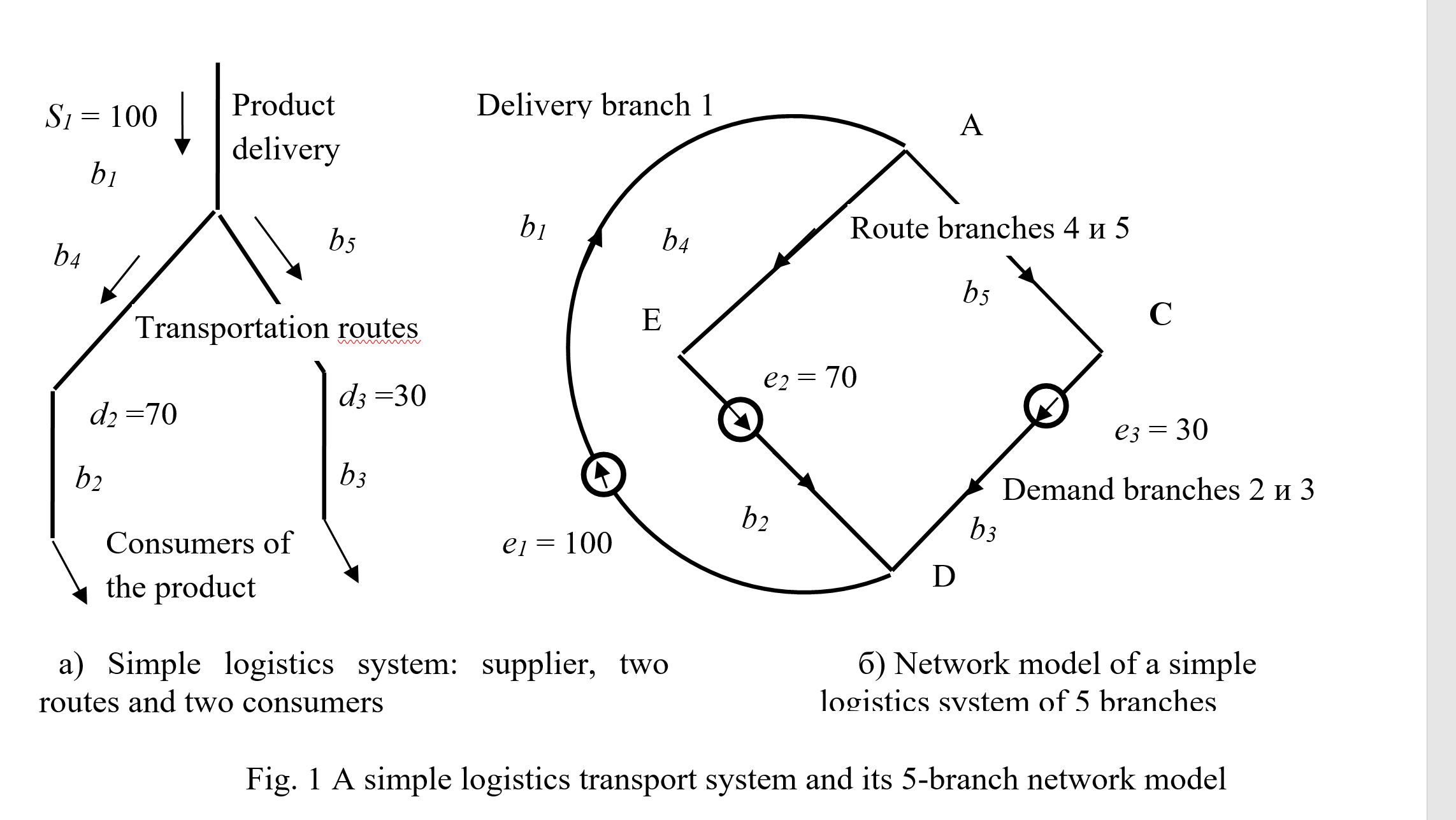
Consider a simple logistics system and the flows in it. There is one supplier, two consumers, two routes in this system and it is shown in Figure 1 on the left. The product flow from the manufacturer of 100 units is delivered via two routes to two consumers receiving 70 and 30 units of the product, respectively. The flows along the routes are equal to the needs of consumers, so their distribution is unambiguous.

The analysis of analogies of the logistics system and the network was carried out in [19], where it was shown that for a simple logistics system presented in Figure 1a, the network model presented in Figure 1b is the most adequate.

The structure of the network model differs from the structure of the logistics system. Since it is assumed that there is an equality of the sum of supplies and the sum of consumption, the input of production and the output of consumption can be considered as "grounding" and link them in one node D.

As a result, two closed paths, contours, which are not present in the logistics system, appear in the network model. It turned out that such a network structure makes it possible to adequately represent product flows in the logistics system. In the network model of the impact, the supply of suppliers and the demand of consumers are represented by voltage sources that are located in the input and output branches.

Suppliers, consumers and the routes connecting them are represented by branches of the network through which product flows, represented by contour currents, pass. Tariffs for storage and transportation of products set the resistance of branches. The specified flows of manufacturers (suppliers) and consumer demand flows are represented by voltage sources e₀. Let the resistances of the branches of suppliers and consumers be equal to units. Then from the equation e₀ = Z i⁰ we get that in a network of separate branches the currents i⁰ = Z^-1 e₀ in the input and output branches are equal to the supply of suppliers and the demand of consumers, and the currents in the branches of routes are zero.

According to the topology of the logistics network, the branches of producers and consumers determine the basis of open paths. The route branches will determine the basis of closed paths in the network. Calculation by formula (1) of the connected circuit network with voltage sources e¹₀ gives currents in the branches of i_c¹, representing, although not completely, the distribution of product flows along the routes. Voltage sources e¹₀ consist of e₁¹₀ - product offerings in supplier branches and e₂¹₀ - product offerings in consumer branches. This solution can be considered as a reference plan, and written as:

i_с¹ = Y_c e₀ = ^mC_t (^mC Z ^mC_t)^{-1 m}C e¹₀,                                                   (5)

where i_с¹ consists of i_1с¹ in the entry branches, i_2с¹ in the exit branches and i_3с¹ in the route branches.

The received currents differ from the set values of supply for i_1с² = i₁⁰ – i_1с¹ and demand for i_2с² = i₂⁰ – i_2с¹.

To supplement up to full product flows, voltage sources are introduced in the branches of the routes defining the basic circuits. These sources should give such currents in the input branches i_1с² and currents in the output branches i_2с², so that they supplement the currents i_с¹ to the set values of the flows of suppliers and consumers. Then the currents i_3с¹ + i_3с² will correspond to the product flows in the routes.

The currents in the input and output branches should be equal to the current difference in the simplest and connected network i_с² = i⁰ - i_с¹, they are created by new voltage sources in routes branches e₃². Additional currents i_3с² in the branches of routes are obtained according to Kirchhoff's law for nodes, route boundaries. Formally, the balance of currents in these nodes is given by the incident matrix M₀¹, connecting nodes and branches, on the basis of which we obtain a system of equations:

M₀¹ i_с¹ = 0.                                                                                (6)

Solving this system of equations, we obtain complement currents only for those routes whose number is equal to the number of basic open paths without unity, i.e. j - 1. For branches of routes representing m basic circuits in excess of this number, i.e. for m - j + 1, the values of the new currents must be set.

The freedom to choose a part of the supplement currents allows you to optimize the choice of routes according to different criteria; assign flows along the selected routes due to certain preferences.

So, the product flows from suppliers, represented by the sum of currents i_1с¹ + i_1с², are distributed along the routes i_3с¹ + i_3с², and arrive at consumers in the right amount i_2с¹ + i_2с², solving the logistics problem. The same problem of the need to introduce additional sources to represent product flows arose during the development of a network model of intersectoral balance [2, 3, 7]. The problem there was solved by using threads in a dual contour network.

The tensor method of network models allows you to calculate flows when the structure changes, including decomposition and calculation in parts of complex networks using efficient algorithms.

The product of the tariffs represented by the resistance of the branches on the product flow gives the cost of transportation along this path, and the sum of all the paths determines the total cost of transportation. By changing the distribution of flows along the paths with the most favorable cost, it is possible to reduce the cost of transportation of goods.

Results of calculation of the network model of the logistics system and discussion

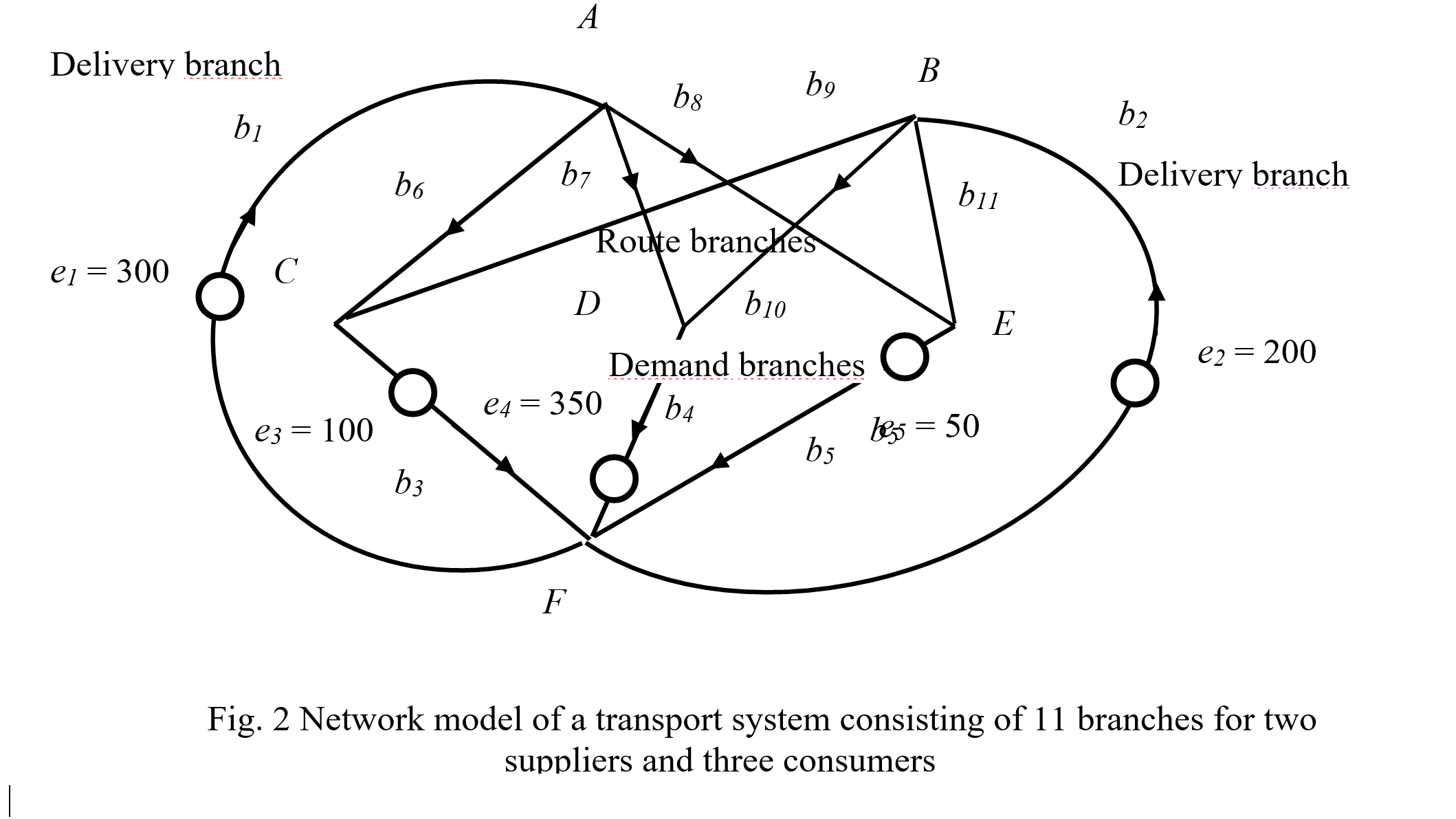
Figure 2 shows an example of a network model of a logistics system, the structure of which is similar to that shown in Figure 1. The network includes two suppliers represented by branches 1 and 2, three consumers - branches 3, 4, 5, which are connected by six routes represented by branches 6 to 11. The resistances of the branches set tariffs, the cost of transporting a unit of product. The calculation is carried out in two stages.

1. Let's define product flows from suppliers in branch 1 - 300 units, and in branch 2  - 200 units; consumer demand in branch 3 is 100 units, 4 - 350, and 5 – 50 units. Supply and demand are represented in the diagram by voltage sources e10.

		1	2	3	4	5	6	7	8	9	10	11
e10	=	300	200	100	350	50	0	0	0	0	0	0	(7)

Six branches of the routes do not yet have sources of impact. The entry and exit branches define open basic paths, the route branches define closed basic paths. Network topology: branches n = 11, nodes J = 6, subnets s = 1, open basic paths j = J - s = 6 - 1 = 5, closed basic paths m = n - j = 11 - 5 = 6.

The transformation matrix describes the structure of transportation of products. The transformation matrix from network paths from individual branches to paths in a connected network, in which the rows indicate the choice of paths, has the form:

		1	2	3	4	5	6	7	8	9	10	11
	1	1	0	0	0	0	0	0	0	0	0	0
	2	0	1	0	0	0	0	0	0	0	0	0
	3	0	0	1	0	0	0	0	0	0	0	0
	4	0	0	0	1	0	0	0	0	0	0	0	jC
	5	0	0	0	0	1	0	0	0	0	0	0
С =	6	1	0	1	0	0	1	0	0	0	0	0	(8)
	7	1	0	0	1	0	0	1	0	0	0	0
	8	1	0	0	0	1	0	0	1	0	0	0	mC
	9	0	1	1	0	0	0	0	0	1	0	0
	10	0	1	0	1	0	0	0	0	0	1	0
	11	0	1	0	0	1	0	0	0	0	0	1

The entry and exit branches define open paths. These are the first five rows that make up the ^jC matrix. The route branches define closed paths – the last six lines, they make up the ^mC matrix. Using the ^mC matrix, we obtain by formula (1) the matrix of the solution of the contour network Y_c.

Let the resistance of the branches be equal to units. Next, we will consider resistances as tariffs for calculating the cost of transportation and storage of products. Then the metric matrix of the basic contours of the connected network has the form: ^mC ^mC_t = z` =

	6	7	8	9	10	11
6	3,0	1,0	1,0	1,0	0,0	0,0
7	1,0	3,0	1,0	0,0	1,0	0,0
8	1,0	1,0	3,0	0,0	0,0	1,0	(9)
9	1,0	0,0	0,0	3,0	1,0	1,0
10	0,0	1,0	0,0	1,0	3,0	1,0
11	0,0	0,0	1,0	1,0	1,0	3,0

By inverting the resulting matrix z`, and multiplying it on the left by <sup>m</sup>C<sub>t</sub>, and on the right by <sup>m</sup>C, we get the solution matrix Y<sub>c</sub> = <sup>m</sup>C<sub>t</sub> (z`)^{-1 m}C =

		1	2	3	4	5	6	7	8	9	10	11
	1	0,625	-0,125	0,167	0,167	0,167	0,208	0,208	0,208	-0,042	-0,042	-0,042
	2	-0,125	0,625	0,167	0,167	0,167	-0,042	-0,042	-0,042	0,208	0,208	0,208
	3	0,167	0,167	0,556	-0,111	-0,111	0,278	-0,056	-0,056	0,278	-0,056	-0,056
	4	0,167	0,167	-0,111	0,556	-0,111	-0,056	0,278	-0,056	-0,056	0,278	-0,056
Yc =	5	0,167	0,167	-0,111	-0,111	0,556	-0,056	-0,056	0,278	-0,056	-0,056	0,278
	6	0,208	-0,042	0,278	-0,056	-0,056	0,514	-0,153	-0,153	-0,236	0,097	0,097	(10)
	7	0,208	-0,042	-0,056	0,278	-0,056	-0,153	0,514	-0,153	0,097	-0,236	0,097
	8	0,208	-0,042	-0,056	-0,056	0,278	-0,153	-0,153	0,514	0,097	0,097	-0,236
	9	-0,042	0,208	0,278	-0,056	-0,056	-0,236	0,097	0,097	0,514	-0,153	-0,153
	10	-0,042	0,208	-0,056	0,278	-0,056	0,097	-0,236	0,097	-0,153	0,514	-0,153
	11	-0,042	0,208	-0,056	-0,056	0,278	0,097	0,097	-0,236	-0,153	-0,153	0,514

Multiply this matrix of the solution by the impact vector given by supply and demand, and represented by voltage sources e¹₀ in vector (7), as a result we get responses, currents in the branches of the contour network ^mi_с¹ at the first stage.

	1	2	3	4	5	6	7	8	9	10	11
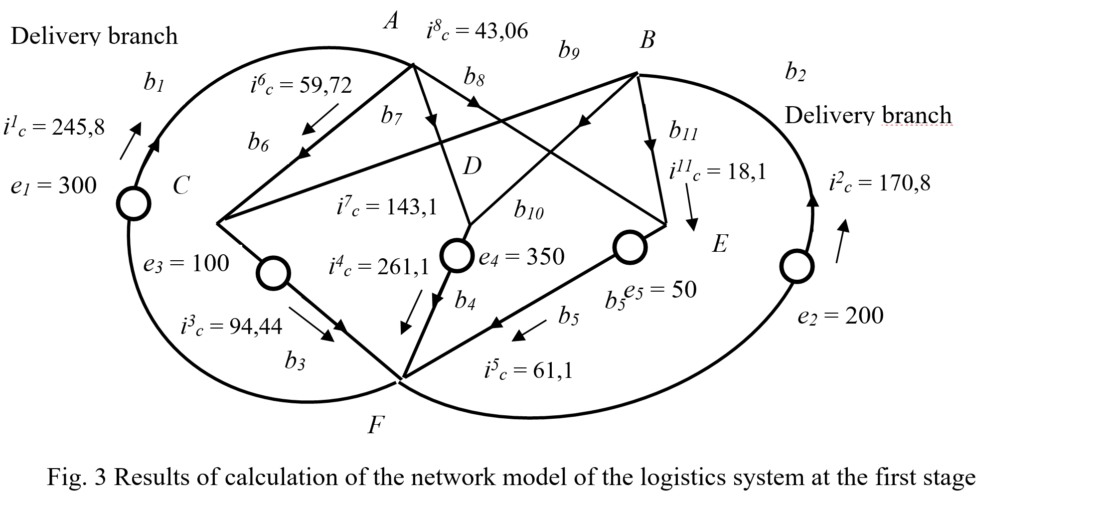
mi1c =	245,83	170,83	94,44	261,11	61,11	59,72	143,06	43,06	34,72	118,06	18,06

Since the resistances are equal to units, the resulting currents in the branches are numerically equal to the voltages on the branches ^mi¹_c = ^me_1c. These are currents that should be analogous to product flows in the logistics network. However, the received response currents to impacts in the input and output branches (warehouses) do not fully correspond to the flows of products that should move from the input to the output.

The results of the calculation of the contour network model at the first stage (currents numerically equal to voltages) are shown in Figure 3.

2. In the network model, the input and output branches define open paths. The basis of closed paths, they are defined by branches of routes, gives independent currents that can be used to construct product flows in a logistics system. It is necessary to find such voltage sources in the branches of the routes, the responses to which will complement the currents obtained at the first stage to the values of the product flows.

Let's denote the number of producer branches n₁, the number of consumer branches n₂, and the number of route branches n₃. The total number of branches n in the network is n = n₁ + n₂ + n₃. There are two nodes in each separate branch. In the network, branches are connected by nodes. Let suppliers be connected to consumers through a grounding node. This means that all manufactured products are delivered to consumers. Then the number of nodes J is equal to the sum of the producer and consumer branches plus one J = n₁ + n₂ + 1. If the route branches have not been added yet, then there are only open paths in the network so far. The number of basic open paths j is equal to

j = J – s = J – 1 = n₁ + n₂ + 1 – 1 = n₁ + n₂,                                       (11)

where s is the number of subnets. Thus, the basis of open paths consists of input and output branches. The branches of routes that connect the outputs of producers with the inputs of consumers add contours, since the number of nodes does not change. Thus, the branches of routes determine the basis of closed paths, the dimension of which is m = n₃. Voltage sources in the branches of routes create additional currents in the network. In sum with the currents obtained at the first stage, they will give values numerically equal to the product flows in the logistics network. First of all, the currents from the sources in the route branches should complement the currents in the input and output branches to the specified supply and demand flows.

The dimension m of the closed path basis may differ from the dimension of the open path basis j. If each input is connected to one output, then the number of routes m will be equal to the greater of the numbers n₁ or n₂. If all inputs are connected to all outputs, then the number of routes will be equal to m = n₁ n₂. This is more than the dimension of the basis of open paths j = n₁ + n₂. Then some contours, their number m - j, should be assigned values. Thus, there is freedom to choose the volume of transportation on some routes, which allows you to optimize, for example, the cost of transportation in this network.

Let's consider the differences between the currents in the individual branches of the network, and those obtained as a result of the calculation of the contour network at the first stage. They correspond to the currents in the node network due to the duality invariant. However, to build product flows, only current differences in the simplest and contour network i_с² = i_с⁰ – i_с¹ in the input and output branches are needed.

Branches	1	2	3	4	5	6	7	8	9	10	11
Currents
In a simple network	300	200	100	350	50	0	0	0	0	0	0
In the contour network	245,83	170,83	94,44	261,11	61,11	59,72	143,06	43,06	34,72	118,06	18,06
Differences	54,17	29,17	5,56	88,89	-11,11	-59,72	-143,06	-43,06	-34,72	-118,06	-18,06

(12)

The currents in the branches at the second stage of the calculation, i_с², are indicated by the branch numbers, for example, i_1с² = 54,17. The i_с² currents in the input and output branches are given, i.e. 1-5, which are obtained as differences in the table. The task is to find new sources, the responses to which will complement the currents in the branches at the input and output to the values of real supply and demand flows. Then, in the branches of the routes, the total currents will give the distribution of the flows of transportation of products from suppliers to consumers. In this case, additional currents in routes, in branches 6, 7, 8, 9, 10 and 11 are unknown. These branches, by virtue of the choice of paths, determine the basis of the circuits in the network structure, and the currents in them are equal to the contour currents.

Additional currents in the branches of routes are obtained from the system of equations (6), where the balance of currents in the nodes according to Kirchhoff's law is expressed in terms of the matrix of incidents, M₀¹ i²_c = 0. This system of equations connects unknown currents in the branches of routes (circuits) and found currents in the branches of open paths. For m – j + 1 currents in the branches of routes, it is necessary to set values, since the current balance equations in the nodes are not enough.

Thus, unknown currents in routes i_3с², in this case, in branches 6-11, can be obtained from the condition of current balance in network nodes A, B, C, D, E and F according to Kirchhoff's law. The incident matrix, M₀¹, for this network has the following form.

	1	2	3	4	5	6	7	8	9	10	11			ic2
A	1					-1	-1	-1					i1с2 =	54,17
B		1							-1	-1	-1		i2с2 =	29,17
C			-1			1			1				i3с2 =	5,56	(13)
D				-1			1			1			i4с2 =	88,89
E					-1			1			1		i5с2 =	-11,11
F	-1	-1	1	1	1

 

Here, on the right, the known currents of the difference in the open paths are given. Multiplying the matrix of incidents by the vector of difference currents, we obtain the following balance equations at the nodes.

Node А: i_1с² = i_6с² + i_7с² + i_8с² = 54,17.

Node В: i_2с² = i_8с² + i_10с² + i_11с² = 29,17.

Node С: i_3с² = i_6с² + i_9с² = 5,56.                                                                                                  (14)

Node D: i_4с² = i_7с² + i_10с² = 88,89.

Node Е: i_5с² = i_8с² + i_11с² = -11,11.

Node F: i_1с² + i_2с² – i_3с² – i_4с² – i_5с² = 0.

In the grounding node F, the balance of the currents of the input and output branches is given. Thus, this node does not participate in the calculation of new currents in the routes. This means that it is necessary to choose values for m - j + 1 currents in the branches of the circuits. In this network of contours m = 6, open paths j = 5, therefore m - j + 1 = 6 – 5 + 1 = 2. It is necessary to set the values of two free currents.

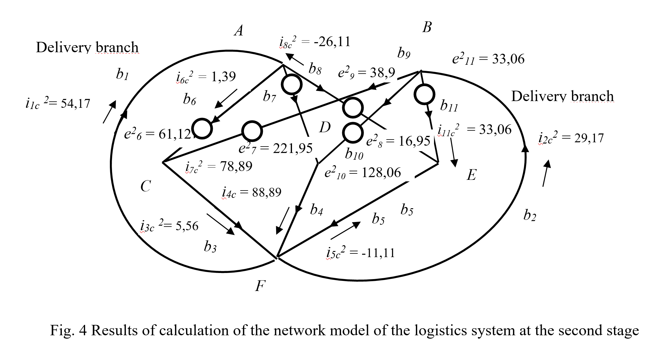
For example, we will set the currents i_10с² = 10, and i_11с² = 15. Solving the balance equations in the nodes, we get the remaining currents in the circuits i^{`</sup><sub>2</sub>: i<sub>6с</sub><sup>2</sup> = 1,39, i<sub>7с</sub><sup>2</sup> = 78,89, i<sub>8с</sub><sup>2</sup> = -26,11, i<sub>9с</sub><sup>2</sup> = 4,17. Multiplying the transformation matrix by the vector of currents in the circuits, we get additional currents in all branches of the network i<sup>2</sup><sub>c</sub> = <sup>m</sup>C<sub>t</sub> i<sup>`}₂ =

	6	7	8	9	10	11				i2c
1	1	1	1	0	0	0			1	54,17
2	0	0	0	1	1	1		i`2	2	29,17
3	1	0	0	1	0	0			3	5,56
4	0	1	0	0	1	0	6	1,39	4	88,89
5	0	0	1	0	0	1	7	78,89	5	-11,11
6	1	0	0	0	0	0	*      8	-26,11	=   6	1,39	(15)
7	0	1	0	0	0	0	9	4,17	7	78,89
8	0	0	1	0	0	0	10	10,0	8	-26,11
9	0	0	0	1	0	0	11	15,0	9	4,17
10	0	0	0	0	1	0			10	10,00
11	0	0	0	0	0	1			11	15,00

The sum of the voltages in the branches of the routes represents the total cost of transporting products. The voltages in the branches of the routes in this case are numerically equal to the values of the contour currents, since they chose that the resistances are equal to units. The values of the voltage sources in the circuits, the basic closed paths, are obtained by the formula, where Z` is given in (9): e<sup>`</sup>₂ = ( ^mC Z ^mC_t ) i<sup>`</sup><sub>2</sub> = Z` i^`₂ =

	6	7	8	9	10	11			i`2			e`2
6	3,0	1,0	1,0	1,0	0,0	0,0		6	1,39		6	61,12
7	1,0	3,0	1,0	0,0	1,0	0,0		7	78,89		7	221,95
8	1,0	1,0	3,0	0,0	0,0	1,0	*	8	-26,11	=	8	16,95	(16)
9	1,0	0,0	0,0	3,0	1,0	1,0		9	4,17		9	38,90
10	0,0	1,0	0,0	1,0	3,0	1,0		10	10,0		10	128,06
11	0,0	0,0	1,0	1,0	1,0	3,0		11	15,0		11	33,06

The sum of the voltage sources located in the branches of the routes is 500.

Figure 4 shows the values of the currents in the branches, which are obtained at the second stage of the calculation, and the voltage sources that create them in the branches of the routes.

The sum of the currents i_c, received in the circuit network at the first stage, i¹_c, and the currents received at the second stage, i²_c is equal to:

		i1c			i2c			i1c + i2c		Sum
	1	245,83		1	54,17		1	300,00
	2	170,83		2	29,17		2	200,00		500
	3	94,44		3	5,56		3	100,00
	4	261,11		4	88,89		4	350,00
ic = i1c  + i2c	=   5	61,11	+	5	-11,11	=	5	50,00		500
	6	59,72		6	1,39		6	61,11			(17)
	7	143,06		7	78,89		7	221,95
	8	43,06		8	-26,11		8	16,95
	9	34,72		9	4,17		9	38,89
	10	118,06		10	10,00		10	128,06
	11	18,06		11	15,00		11	33,06		500,01

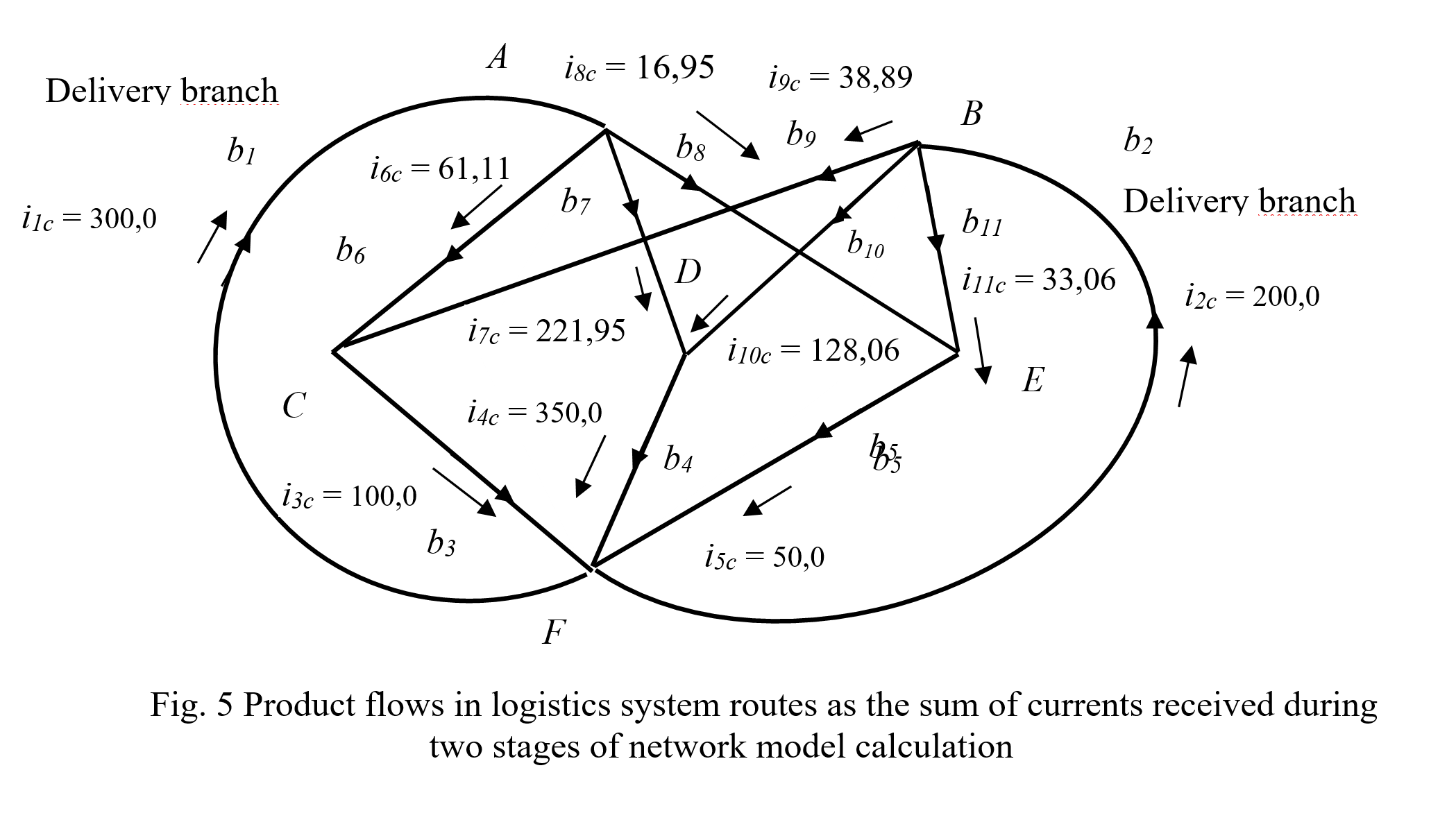
It is shown on the right that the sum of currents in the input and output nodes is 500, which corresponds to the specified flow of supply and demand, which are distributed along the branches of the routes. The sum of flows along the routes is equal to the sum of flows at the input and the sum of flows at the output, namely, is equal to 500, taking into account rounding, i.e. all product flows are delivered.

Figure 5 shows the values of the currents in the branches, which represent the sum of the currents obtained by two stages of calculation (17). Voltage sources are not shown.

At the same time, other options are possible, setting requirements for certain routes. For example, let's assign currents in the other two branches of the routes i_6с² = 20, i_7с² = 30. The following results are obtained:

Branches	1	2	3	4	5	6	7	8	9	10	11
i1c	245,83	170,83	94,44	261,11	61,11	59,72	143,06	43,06	34,72	118,06	18,06
i2c	54,17	29,17	5,56	88,89	-11,11	20,00	30,00	4,17	-14,44	58,89	-15,28
i1c + i2c	300,00	200,00	100,00	350,00	50,00	79,72	173,06	47,23	20,28	176,95	2,78

At the first stage, the results are the same, but the sum of currents representing the distribution of product flows along the routes turned out to be different. The choice of values of free currents is limited by the fact that the product flows must be non-negative. However, negative values can be interpreted as the need to return products that have already been delivered in order to meet the assigned requirements.

The sum of flows along the routes is also equal to the sum of flows at the input and output, i.e., equal to 500, taking into account rounding, i.e. all product flows are delivered. The network model allows the decomposition and calculation by parts of complex systems using algorithms developed in the tensor method of dual networks.

The network model provides the calculation of the cost of transportation. By analogy, we will assume that tariffs are represented by branch resistances. Then the voltages on the branches represent the cost of transporting the flow of products along this route. The sum of the voltages (costs) on all routes gives the total cost of transporting products.

As an example, we will assign tariffs as resistances in the branches of routes, which for brevity we will represent as a vector, although in reality this is the main diagonal of the resistance matrix. The voltages on the branches will be obtained by the formula e¹_c + e²_c = Z (i¹_c + i²_c).

Branches	1	2	3	4	5	6	7	8	9	10	11
Z	1	1	1	1	1	2	3	4	5	2	3
i1c	185,1	141,5	81,8	195,9	48,9	66,5	89,6	29,0	15,3	106,3	19,9
i2c	114,9	58,5	18,2	154,1	1,1	-15,3	139,1	-8,7	33,5	15,0	10,0
i1c + i2c	300,0	200,0	100,0	350,0	50,0	51,2	228,7	20,3	48,8	121,3	29,9
e1c + e2c	300,0	200,0	100,0	350,0	50,0	102,3	686,1	81,3	244,2	242,6	89,6

The sum of the voltages in the branches of routes 6 to 11 is equal to 1446,14; this is the total cost of transporting products at the specified supply, demand, and tariffs. For comparison, let's consider another option for setting tariffs with the Z matrix, the main diagonal of which is represented by a string.

Branches	1	2	3	4	5	6	7	8	9	10	11
Z	1	1	1	1	1	6	4	2	3	2	2
i1c	163,1	151,2	59,4	183,5	71,4	29,6	75,8	57,7	29,8	107,7	13,7
i2c	136,9	48,8	40,6	166,5	-21,4	16,8	151,5	-31,4	23,8	15,0	10,0
i1c + i2c	300,0	200,0	100,0	350,0	50,0	46,4	227,3	26,3	53,6	122,7	23,7
e1c + e2c	300,0	200,0	100,0	350,0	50,0	278,2	909,4	52,6	160,9	245,3	47,4

 The sum of the voltages in the branches of routes 6 to 11 is 1693,76; this is the total cost of transporting products when setting new tariffs. The change (redistribution) of tariffs led to a different distribution of flows along routes and the total cost of transporting products.

 

Conclusion

The created network model of the logistics system based on the tensor method of dual networks provides the calculation of product flows along routes from suppliers to consumers in two stages without iterations, as well as the calculation of the cost of transportation in accordance with tariffs. To analyze the options, you can select the parameters of supply and demand, fare values, route schemes, etc.

A certain limitation of the logistics network model is the need to specify at the second stage of the calculation the values of currents in some branches of routes, the number of which is equal to the difference between the dimension of the closed path basis and the open path basis. The model provides the calculation of the transportation plan when new requirements arise for the volume of transportation along certain routes using path transformation matrices. Variations in the route structure and supply and demand parameters need to be used to optimize the transportation plan, which requires further research.

The further direction of research will be the application of decomposition and calculation by parts of complex logistics systems, calculation of flows when changing the structure of routes using algorithms of the tensor method of dual networks, analysis of the behavior of the system when changing the tariffs for storing products.

1. Kron G. Diakoptics – the piecewise solution of large-scale systems. MacDonald, London, 1965.
2. Petrov A.E. Tensornaya methodologiya v theorii system [Tensor methodology in the theory of systems]. - M.: Radio i Sviaz = M.: Radio and Communications, 1985. - 152 p. (In Russ.).
3. Petrov A.E. Tensornyi method dvoistvennyh setei. [Tensor method of dual networks]. Moscow: Cetis LLC. http://устойчивоеразвитие.рф/files/monographs/Petrov_Tenzorny_method.pdf – 2009. – 496 p. (In Russ.).
4. Petrov A.E. Logistica v SAPR [Logistics in CAD]. Part 1. Logistica proizvodstva [Production logistics]: educational and methodical manual Moscow: МГГУ, 2012. – 92 p. http://window.edu.ru/resource/548/79548 https://www.twirpx.com/file/1193744/ – 2012. Part 2. Informationnaya Logistica [Information logistics]: educational and methodical manual Moscow: МГГУ. – 112 p. https://window.edu.ru/resource/549/79549 – 2013. (In Russ.).
5. Obraztsova R.I., Kuznetsov P.G., Pshenichnikov S.B. Engineerno-economiceski analys transportnyh system. Methodologia proektirovania automatizirovanoy systemy upravlenia. [Engineering and economic analysis of transport systems. Methodology of designing an automated control system] / Под. Ред. К.В. Фролова.- 2-е изд. Стереотип. – M.: Radio and Communications, 1996. – 192 p.: илл. – ISBN 5-256-01342-4. (In Russ.).
6. Petrov A. E. Zakon sohrayenia mochnosti v dvoystvennych tenzornyh setyah G. Krona - A. Petrova (v prostranstve, vremeni i structure). [The law of conservation of power in dual tensor networks of G.Kron - A.Petrov (in space, time and structure)]. Electronic scientific publication "Sustainable Innovative development: Design and management", ISSN 2075-1427. volume 15 No. 1 (42), 2019, art. 1. - pp. 1-39. http://www.rypravlenie.ru/?p=3356. (In Russ.).
7. Petrov A.E. Network methods of production planning: educational and methodical manual. Moscow: MGSU. https://window.edu.ru/resource/545/79545/files/Petrov_methods.pdf. – 2010. – 144 p. (In Russ.).
8. A.E. Petrov. Tensor Method and Dual Networks in Electrical Engineering. ISSN 1068-3712, Russian Electrical Engineering, 2008, Vol. 79, No. 12, pp. 645–654. © Allerton Press, Inc., 2008. ISSN 1068-3712, https://pdfslide.net/documents/tensor-method-and-dual-networks-in-electrical-engineering.html. Original Russian Text © A.E. Petrov, 2008, published in Elektrotekhnika, 2008, No. 12, pp. 2–12.
9. Petrov A. E. The duality of networks for computer-aided design systems with variable structure. Mining Informational and analytical bulletin (scientific and technical journal). Reports of the XXIII International Scientific symposium «Miner's week – 2015» Collection of scientific tr. Publishing House of NUST MISIS. ISBN 987-5-87623-891-7. – 2015.
10. Petrov A.E. Tensornyi metod dvoystvennyh setey dly rascheta slognyh system po chastyam. [Tensor method of dual networks for calculating complex systems in parts]. - UDC: 338.26.015: 658.5, Moscow: Publishing House "Mountain Book". pp. 168-192. Moscow: MGSU, Mining Information and Analytical Bulletin (scientific and Technical journal), 2017. (In Russ.).
11. Bolshakov B.E., Petrov A.E. Algorithms of Multidimensional Space and Time Values Interrelation in the System of LT Dimension Coordinates by B. Brown, R.O. Bartini, P.G. Kuznetsov. Journal of Engineering and Applied Sciences, Pakistan, 2017, 12: pp. 6620-6627. DOI: 10.36478/jeasci.2017.6620.6627. https://medwelljournals.com/abstract/?doi=jeasci.2017.6620.6627
12. Korolkova, M. A. Optimizatia seti avialinyi na osnove tensornoy methodology. Abstract of the dissertation for the degree of Candidate of Technical Sciences, St. Petersburg, 2003. (In Russ.).
13. Sokhor, Yu.N. Tensorniy analys setey i diacoptica v enginernih radchetah. / Yu.N. Sokhor. - M.: LAP Lambert Academic Publishing, 2012. - 200 p. (In Russ.).
14. Voronov P.L. Features of the application of transformation matrices and coupling equations in the analysis of asymmetric damages. Bulletin of the South Ural State University. Ser.Power Engineering. 2018, vol. 18, no. 1, pp. 27–37. (In Russ.).
15. Lyamets, Y.Ya. Equivalence of multi-wire systems with short circuits and breaks of part of the wires / Yu.Ya. Lyamets, D.G. Eremeev, G.S. Nudelman // Electricity. - 2003. - No. 11. - pp. 17-27. (In Russ.).
16. Shvetsov V. I. Mathematical modeling of transport flows//Automation and Telemechanics, 2003, Vol. 11, P. 3-46. (In Russ.).
17. Cascetta. Transportation Systems Analysis. Models and Applications. Springer, 2009.
18. Petrov A.E. Diacoptics of the structure of transport networks – XVI All-Russian Scientific Conference "Neurocomputers and their application". Abstracts of reports M.: MGPPU - 2018 - pp. 315-317. ISBN 978-5-94051-136 6.https://it.mgppu.ru/upload/iblock/b35/НКП%20XVI%20%20тезисы.indd%20(1).pdf. (In Russ.).
19. Petrov A.E. Network model of logistics system // Online scientific publication "Sustainable innovative development: design and management". 2021. Vol. 17, issue 3 (52). - pp. 1-20.URL: http://www.rypravlenie.ru/?p=3792. (In Russ.).
20. Bogdanova L.V. Discrete tensor analysis in railway transport. In the collection: Proceedings of the international scientific and practical conference "Prospects for the development and efficiency of the functioning of the transport complex of the South of Russia". In 3 parts. Rostov State University of Railway Transport. 2015. pp. 81-83. (In Russ.).
21. A.E. Petrov, A.V. Fedorov, A.V. Kochegarov, E.N. Lomaev, A.P. Preobrazhenskiy. The Analysis of Network Models for the Design of Industrial and Fire Safety Systems for Oil Refineries. IOP Conf. Series: Earth and Environmental Science 808 (2021) 012024, IOP Publishing doi:10.1088/1755-1315/808/1/012024.
22. Litvinov K.A., Pasechnikov I.I. Algoritm rascheta tenzornoy modeli seti na osnove simpleksnogo metoda dantsiga. [Algorithm for calculating the tensor model of the network based on the simplex Danzig method]. Bulletin of the Tambov University. Series: Natural and Technical Sciences. 2013. Vol. 18. No. 6-2. pp. 3370-3375. https://cyberleninka.ru/article/n/algoritm-rascheta-tenzornoy-modeli-seti-na-osnove-simpleksnogo-metoda-dantsiga. URL OF THE RSCI: https://elibrary.ru/item.asp?id=21106190. (In Russ.).
23. Kamzolov Dmitry. Near-Optimal Hyperfast Second-Order Method for Convex Optimization. MOTOR 2020 Communications in Computer and Information Science (CCIS) 1275 proceedings, pp. 1–12, 2020. https://doi.org/10.1007/978-3-030-58657-7_15.
24. Dmitry Kamzolov, Alexander Gasnikov and Pavel Dvurechensky. On the Optimal Combination of Tensor Optimization Methods. OPTIMA-2020 proceedings in Lecture Notes in Computer Science (LNCS). Springer. Volume number 12422.
25. Zaitsev E. I., Bochkarev A.A. Model functionalnoy i structurnoy nadegnosty cepi postavok. [Model of functional and structural reliability of the supply chain]. // Logistics and Supply Chain Management: Modern Trends in Germany and Russia: tez. dokl. IV German-Russian Conference on Logistics and Supply chain management (May 6-9, 2009). Göttingen: Cuviller Verlag, 2009. pp. 187-195. (In Russ.).
26. Morozov A.V., Ponomarev D.Y. Model raspredelenia raffica v mnogourovnevoy infocommunicacionnoyseti specialnogo naznachenia. [Traffic distribution model in a multi-level info communication network of special purpose]. Modeling, optimization and information technology. 2021. vol. 9. No. 1 (32). pp. 11-12. (In Russ.).
27. A.A. Luk'yanchenko, A.E. Petrov, A.V. Fedorov, A.N. Denisov. Method of Rational Location of Gas Detectors For Early Fire Detection Based On Gas Control Technology. Jour of Adv Research in Dynamical & Control Systems, JARDCS, USA, Vol. 12, Issue-06, 2020. Pp. 1293–1306. DOI:10.5373/JARDCS/V12I2/S20201321.. https://jardcs.org/archivesview.php?volume=3&issue=36&page=6.