Synthesis and identification of hidden Markov models based on a novel statistical technique in condition monitoring

1.          INTRODUCTION

Jet engine noise, pressure fluctuations in turbulent boundary layer and other high-level acoustic loads result in fatigue failures of aircraft structures. These problems have been attracting attention of researchers since the 1950s after numerous acoustic fatigue failures of aircraft resulted from airspeed increase and changed engine types. In recent years, the interest to this problem has greatly increased owing to a new generation of supersonic airplanes and hypersonic flight vehicles developed.

Acoustic loads are the most dangerous for thin-walled aircraft structures. These loads are wide-band (up to 5000 Hz) random process, with level varying from 145 dB to 170 dB in different points of aircraft surface.

In practice, destructiveness of these structures can be estimated by the changes of distributed structure stiffness, which is, in its turn, recognized by the qualitative changes of normalized spectral structure characteristics measured in checkpoints. Normalizing makes it possible to analyze only qualitative response and not to take into account the level of load. Such an approach based on the estimation of averaged structure properties seems more promising than the direct search for separate cracks[6,18], which are not always accessible for direct observation and hard to forecast because of considerable dispersion in their evolution. The use of secondary characteristics (such as spectra) instead of time-domain realizations as check data is caused by the following facts:

-       Spectra keep a sufficient amount of useful information about processes under study

-       Spectra need less memory in digital representation

-       Spectra may be easily and quickly computed with controlled accuracy.

Structure diagnostics and service life forecasting are two important technical problems to be solved during condition monitoring of aircraft structures suffered fatigue failures. Their solution is necessary for both planning maintenance works and estimating destruction level. The results obtained give the opportunity to cut down expenses for aircraft maintenance, raise the reliability of destruction monitoring, simplify the routine maintenance and derive its more justified schedules. Technology for monitoring of fatigue failures based on capabilities of neural[2] and discriminant networks was considered in papers and books[1,9-12,15].

As it was shown in the book[5], probabilistic models of cumulative damage are more preferable for forecasting in the discussed area than the deterministic ones. A relevant approach founded on Markov process theory was presented in works[1,9-10,12,14-15].

According to this approach, forecasting is based on accumulated observations. Probability dynamics is described by continuous time, discrete state Markov processes. The given damage types are considered as separate discrete states in which the analyzed system has some probability to find itself. In due course transitions between the states are the case. It is assumed that state-to- state transitions (corresponding to each branch of the graph) meet the properties of Poisson flows of events. Time-domain dynamics of state probabilities is described by Kolmogorov set of ordinary differential equations.

Transition flow rates are free model parameters. Comparison of observed and expected histograms which present observed damage distributions at given time points, is used to identify them. The technique to find independent parameters as those minimizing a certain goodness-of-fit measure is used. According to the given approach, this measure is minimized at the specified time points, in which observed data are available. The employed procedure of parameter estimation as well as its software implementation were described in books[1,15]. In fact, an inverse problem is solved, viz.: coefficients of differential equations are determined by using the given solution characteristics. Obtained values of free parameters are considered as fatigue failure characteristics which have become apparent during observations.

It was shown that Markov models under the given inverse problem formulation may be regarded as specialized neural networks. The technique for their synthesis to select the most suitable network structure was developed on the base of statistical criteria[1,13,15]. Proposed in papers[12,14] was further development of this approach, the concept of multifactor Markov networks to represent subtle features of cumulative damage development and improve concordance between observed and predicted behavior. The papers mentioned present new features of these trained structures, including their 3-D applications, and show advantages of probabilistic predictions obtained with the aid of Markov networks to improve the damage diagnostics quality. Markov models in question make it possible both to forecast probabilities of damage types and identify them on the base of observed system characteristics. Thereby they fix up typical condition monitoring problems solution for the structures under study.

Taking into account indirect observations for the system states, Markov networks under the given problem formulation can be considered as a special case of continuous-time hidden Markov models, which use measured spectral characteristics in checkpoints as observed parameters and are obviously regarded as more difficult instruments for practical applications than the traditional discrete time ones.

As for the structure service life forecasting in case of an identified Markov network, damage state probabilities as functions of time are obtained by means of integrating Kolmogorov set of differential equations. This operation is not difficult and is beyond the application field of hidden Markov models.

In its turn, diagnostics of the technical systems under consideration, which suffer damages of different types, is carried out in case of uncertainties when neither possible defect types nor connections between them are known beforehand. There is no information about the damage framework of such systems since:

-       Some defects may not be identified easily and quickly (particularly, when it is difficult to get access to a structure part or find cracks because of their small size)

-       Defects are usually not monitored directly and may be revealed by implication only via the system characteristics which are available for measurements (for example, spectra in checkpoints)

-       Strict reasons for damage discrimination are frequently absent

-       Experimental estimation of mutual connections between different defect types is a labor­intensive and long process, as a rule.

Two principal problems are usually to be solved to support structure diagnostics of the given ambiguous systems represented by the aforementioned probabilistic models:

-       Given the parameters of Markov model in use and a particular sequence of observed spectral characteristics in structure checkpoints, find the sequence of different damages represented by model states, which is most likely occurred (identification problem)

-       Given observed spectral characteristic sequences, find the most probable Markov model for representation of damage framework including the set of states, the structure of transitions between them and quantitative parameters of these transitions (synthesis problem).

Thus, the problem of constructing hidden Markov models best conformed with observations in case of uncertainties has been arisen. Presented in this paper are technologies for synthesis and identification of Markov models based on a novel statistical identification technique which can be applied for both continuous- and discrete-time models.

The given approach is intended for solution of both problems specified before. When solving the synthesis problem it determines a set of relevant states, their connections and optimal values of free model parameters for Markov networks. Some features of this technique were described in pa- pers[12-13] and books[1, 15]. If discrete-time structures (Markov chains) fit an application problem better (for example, in case of discrete-time output of observed spectral characteristics with certain sampling interval), conversion from an initial continuous-time structure to the corresponding discrete-time one is carried out with the aid of a suggested special procedure.

Owing to universality and flexibility, the presented way of solution has obvious advantages over the methods used for maximum likelihood estimation of parameters for traditional hidden Markov models represented by Markov chains given a dataset of observed output is available. Until recently, no tractable algorithm has been known to solve such a problem, but for the Markov chains a local maximum likelihood can be efficiently derived by using Baum-Welch or Baldi-Chauvin al- gorithms[2,19]. It should be noted that the presented way of solution calculates not only optimal values of free model parameters like Baum-Welch and other algorithms but, in addition to this, a set of relevant states and their connections. It is significant that traditional algorithms for hidden Markov models are unable to solve the applied technical problem considered here when uncertainties with damage types, model states and their connections are the case or the number of sampling points is too small.

Solution of the identification problem requires to find the most probable damage sequence over all the possible ones, with the probabilities of certain observed spectra belonging to given states in use. In case of Markov chains, the solution of interest can be found by Viterbi algorithm[20] but, taking into account a relatively low number of model states in many application problems, exhaustive search algorithms are also acceptable for solution in case of both continuous-time and discrete-time models.

In spite of the technology in question is considered here in application to a particular technical problem, the presented mathematical tools are not fastened to the given field of use and can be exploited for solution of many other technical and non-technical tasks. In particular, the conversion of discrete-time models to continuous-time models with their following identification and return to the initial structure is highly promising allowing for greater capabilities for model synthesis in continuous-time domain.

2.          SOLUTION TECHNOLOGY

2.1.    Synthesis problem

The synthesis problem solution includes the following stages:

1)     Reduction of input data dimension to remove the redundant information

2)     Determination of a set of states for Markov network via either Kohonen classification with the aid of Kohonen self-organizing feature maps (Kohonen maps) or multivariate clusteriza­tion procedure

3)     Determination of initial distribution of connections between the states according to either contiguity of activated parts of Kohonen maps or multidimensional scaling

4)     Adjustment of connections (removing redundant and statistically insignificant connections) by means of successive identification of transition flow rates by the chi-square minimum method

5)     Final identification of network parameters by the chi-square minimum method.

2.1.1.    Input data

As is shown in paper[9], it is convenient to estimate the level of fatigue failure for the structures suffered damages via response power spectral densities measured in checkpoints. These spectra are further considered as initial analyzed data. It is assumed that some representative sample of spectra resulted from either structure tests or observations during operation is available, with a damage type being specified for only certain of the spectra. Power spectral densities are regarded to be calculated with the accuracy sufficient for qualitative recognition[3].

2.1.2.    Reduction of input data dimension: Synthesis stage 1

In case of observed data represented by spectral characteristics measured in structure checkpoints it is expedient to bring analyzed variables to conformity with frequency ranges taken with a certain step. Values of these variables are averaged normalized spectral characteristics for the corresponding frequency ranges. A large number of input variables, which is typical for this representation, may complicate the input sample analysis: in particular, the number of observed data necessary for qualitative network synthesis may become too great. Solution of this problem by worsening the spectral resolution capability is unacceptable as the useful information is lost. It is possible to improve the analysis quality only if the input data dimension is eliminated at the expense of redundant or insignificant information.

The ways of this problem solution are considered in paper[9] and books[1,15]. The method of principal components[16] is the most suitable among the permissible variants since it is the simplest and does not require any special assumptions on the initial data. The given approach makes the results of analysis independent of the spectrum evaluation features.

2.1.3.    Determination of a set of states for Markov network: Synthesis stage 2

A set of Markov network states is determined by classifying the damage types: its own state corresponds to each type. As the damages for input cases are assumed to be partially known, it is necessary to propagate the given classification to the spectra which have no assigned damages to. Two alternative instruments can be used to determine the model states: Kohonen maps or multivariate clusterization.

The classification propagation method based on Kohonen maps contains the following steps: 1) Select Kohonen map[8], where the number of elements exceeds considerably the expected number of damage types.

2)    Train the network by using input cases for which damages are known. Mark the neurons of the topological map, which won for one damage type only. (Labels correspond to damage types.)

3)    Input the remaining part of the sample to the network. Attribute the damage labels to the input cases, for which the marked neurons win.

4)    If a subset of input cases, for which damages are known, is extended, then go to Step 2 else stop the computation.

If the sample of input cases still contains elements with unknown damages, the following actions are possible:

-        Provide the network with a special state Unknown for unknown damages and attribute unclassified elements to this type (see Section 3);

-        Undertake the structure inspection and classify the remaining elements of the sample (if their number is not too great).

It is expedient to carry out clusterization in four steps:

1)      Tree clustering to get hierarchical tree plot and estimate reasonable number of clusters which are used later to form the model states[4] (in case of input data discussed before, the Ward’s method with Euclidean distances is recommended)

2)      K-means clustering for the number of clusters determined at the previous step to find out the content of each cluster

3)      Assigning proper labels to clusters which contain the predominant number of marked elements of a given damage type

4)      Meshing clusters with identical labels to higher-level clusters corresponding to a given damage type (optional).

1.1.4.    Determination of connections between the states of Markov network: Synthesis stage 3

To determine initial distribution of connections between Markov network states, information on contiguity of activated parts of Kohonen maps or analysis of multidimensional scaling results can be used.

In the first case the associative properties of Kohonen maps are used, viz.: similar cases activate the groups of closely set neurons. Connections between the states are predicted according to contiguity of activated areas of the marked topological map. Each of these areas corresponds to a fixed damage type (Figure 4).

The formal rule to find out contiguity of the areas is not unique. One of the convenient ways is to count minimal distances between pairs of marked neurons in Manhattan metric. Used for comparison are minimal distances between two differently marked neurons:

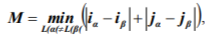
where L(a) and L(β) are labels of neurons with the a and β indices; indices a and β take all the values meeting the indicated condition; i_a and i_p are numbers of rows, in which the neurons with indices a and β are disposed at the topological map; j_a and j_β are corresponding numbers of columns. Those and only those pairs of states p and q are supposed to be adjacent, for which the following condition is the case:

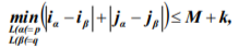
where indices a and β take on all the values that meet the indicated conditions; k>0 is the integer­valued parameter (in standard conditions k may be equal to zero).

Multidimensional scaling is applied to a matrix of Euclidean distances between the centers of clusters which correspond to different damage types and were determined at the previous step. As a result, these centers are usually inserted into two- or three-dimensional space. Possibility of transitions between the model states is derived from the values of distances between them. Thereby, the hypothesis of transition possibility dependence on distance in the obtained space is used.

When forming an initial Markov model structure, each state is connected with the states which centers are at the minimal distance from its center or at the distances exceeding the minimal one less than the given percent (in practice the 50%-limit may be recommended). The cluster center corresponding to the normal system operation is represented by the initial state. Directions of transitions along state connections are determined according to proximity to the initial state, viz.: transition from one state to another is possible if they are connected and the minimal number of transitions from the initial state to the first one is less than the analogous/similar number of transitions to the second one. If direction is ambiguous, both variants of transitions are attributed to the corresponding connection.

The structure obtained as a result of any given procedure takes into account redundant and statistically insignificant connections, which are revealed and removed at the next stage of calculations.

1.1.5.     Adjustment of connections: Synthesis stage 4

In training the network, its free parameters are selected to get the best correspondence between observed and expected histograms of being in the system states at the given time points. Pearson statistic

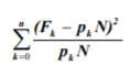
is used as a goodness-of-fit measure, where F_k is observed frequency of getting into the k-th system state at a given time point, p_kN is corresponding expected frequency, p_k is expected probability of being in the k-th state, N is the sample size, n is the number of model states. The smaller the value of this statistic the better the correspondence between observed and expected results. Under some conditions[7], it is distributed asymptotically according to a chi-square distribution. Expected state probabilities are obtained by means of numerical integrating Kolmogorov set of differential equations.

The given technique of identifying free parameters is called the chi-square minimum method. For the problems under consideration, it yields estimations which are close to the ones obtained by the maximum likelihood method[7]. It was proved that, under some general conditions, Pearson statistic values derived by substituting the indicated solutions were described asymptotically by the chi-square distribution with n-s-1 degrees of freedom, where s is the number of free parameters to be determined, with the calculated values of free parameters converging in probability to the desired solution when increasing the sample size[7]. These facts allow to use the given statistic for testing the hypothesis of agreement between observation data and Markov network forecast.

The procedure for finding optimal values of free parameters, which is based on electronic spreadsheet capabilities, is considered in works[1,9,15]. It was also shown there how to optimize the model, using statistical goodness-of-fit tests.

Adjustment of connections in Markov networks (viz.: removing indirect and statistically insignificant connections) is carried out on the basis of the same approach. A network, in which all the transition flow rates are free parameters, will be called the complete network. Networks, in which some conditions are imposed on free parameters (for example, the conditions of equality to zero), will be called the reduced networks. The hypothesis of agreement between obtained observation data and a complete Markov network forecast will be denoted as H_c.

If there are no reasons to reject hypothesis H_c, each network connection tests of the significance are carried out in turn. For this purpose, free parameters are evaluated by the chi-square minimum method under the condition of flow rate equality, which corresponds to the connection tested, to zero. Obtained value X_r² of Pearson statistic is compared with the analogous characteristic X_c² for the complete network. Since difference  is asymptotically distributed as a chi-square with 1 degree of freedom[4], this statistic is used for testing null hypothesis H_r of the agreement between the observation data and the reduced network forecast against the alternative hypothesis H_c. If hypothesis H_r is not rejected at the given significance level, the corresponding connection is marked as a candidate for withdrawal from the network.

It is expedient to refine the network by iterations, using a sufficiently great value for the significance level, at which a connection is removed (p=0.5 is recommended), and a small value for the significance level at which a connection remains in the network (p=0.01 is recommended). The result obtained after removing connections at the current stage of calculations is considered as a complete network at the following iteration. Under such conditions, only a fortiori redundant connections are withdrawn from the network after each iteration (p>0.5). Solution with regard to questionable connections (0.01 <p < 0.5) is postponed. As a rule, significance of questionable connections is clarified step-by-step. This fact is caused by simplified network under study.

1.1.6.    Final identification of network parameters: Synthesis stage 5

At this stage, free parameters of the obtained network are identified by using the chi-square minimum method. The goodness-of-fit for observed data and forecast is estimated by the minimal value of Pearson statistic. Number of degrees of freedom for the chi-square goodness-of-fit test is determined as a difference between the number of independent observed statistics F_k and the number of parameters to be found.

2.2.    Identification problem

The number of sampling instants q, at which spectral characteristics in structure checkpoints are estimated, should be selected beforehand for the identification problem solution. The identification procedure includes the following steps:

1)     Determination of all the model state sequences  which are possible for developing a system under study during a given number of sampling instants

2)     Estimation of occurrence probabilities P(S_i) for every sequence  indicated at the previous step via the product of probabilities of transitions between the model states during in- q-1

tervals limited by the given sampling instants in the following way: , where u=1

is probability of transition from state s_iu occupied at instant u to state s_i,u+1 occupied at instant u+1. These transition probabilities can be calculated by using either Markov chains or Markov networks[5]

3)    Estimation of occurrence probabilities P_iz of observed sequence of spectral characteristics in structure checkpoints for state sequences in the following way:

is probability of acquisition of observed characteristic z_j be- j=1

ing at state

4)    Selection of the most probable state sequence corresponding to the maximal probability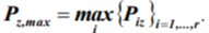

When sampling estimations of distribution parameters for the distances of observed data corresponding to each model state from state centroids[7] of these data are available, it is expedient to replace quantities  by probability density functions  of Euclidean distances xj of characteristics zj from the observed data centroids for corresponding states sij[8]. It is the distance parameter that determines estimations of occurrence probabilities for observed characteristics in this case.

It is necessary to note that Markov chains are more convenient for identification than Markov networks since they ensure simpler calculations. In its turn, Markov networks are more convenient for synthesis of hidden models owing to their greater flexibility and capabilities of problem solution when only a few observation instants are available and model states are unknown a priori.

2.3.    Conversions from continuous-time models to discrete-time models

Conversions from a continuous-time model to the corresponding discrete-time one and vice versa are carried out if this is expedient for the application problem solution. Conversion to a continuous­time model is in fact determined by a proper mapping of a sequence of Markov chain discrete steps onto Markov network continuous-time scale. In case of inverse conversion, the following procedure is suggested:

1)    Selection of a sampling interval т on the continuous-time scale, which corresponds to the discrete step of Markov chain

2)    Integration of Kolmogorov set of differential equations describing the state probability dynamics in an initial Markov network to calculate, as a result, the sequence of probability distribution vectors Pi (i=0,1,...,l) corresponding to a given sequence of l+1 discrete time points taken with the selected sampling interval т

3)    Construction of transition probability matrix A=||aij|| of order nxn, where n is the number of states of Markov chain under consideration which represent this chain dynamics with the aid of free variables denoting transition probabilities and, if necessary, analytical expressions assembled from these variables

4)    Numerical solution of multivariate optimization problem with the following conditions to estimate required values of free variables which matrix A are composed of:

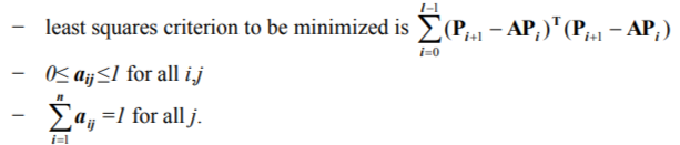
Obtained values of the specified free variables yield the sought transition probability matrix A that determines state changes of Markov chain in question: P;+x = AP, i=0,1,...,l. Statistical significance of relevant residual error can be evaluated by means of obviously modified Pearson statistic (see Section 2.1.5).

3.          APPLICATION EXAMPLE

The proposed technique features are shown by the example of synthesis and identification of Markov models representing fatigue failures of an aircraft air-intake panel. Its characteristics and damage types are presented in works[1,10].

Observation data were represented by a sample of 144 pairs of stress power spectral densities measured at two checkpoints in the range from 500 to 2500 Hz. Some patterns of these characteristics are given in Figure 1. Damage types were supposed to be known beforehand for 25 spectral pairs only. Spectra for the test sample of air-intakes were estimated after 1000 and 2000 exploitation hours. Six damage types were identified. Each observed case contained average values of normalized spectral densities in 45 frequency ranges of 45-Hz width. Thus, the initial set of data to be analyzed included 90 input variables.

After reducing the problem dimension by the principal component method, the number of input data was diminished up to 10 variables, which were used in the following analysis (10 first principal components explained more than 80% of observed variance).

The method of classification propagation made it possible to expand the identified part of the sample up to 115 elements by two iterations. The Kohonen map composed of 25 units was used (Figure 2). For five pairs of spectra, the damage types were determined by the additional inspection. 24 pairs of spectra remained unclassified. The Kohonen maps work was simulated with the aid of the STATISTICA Neural Networks software package.

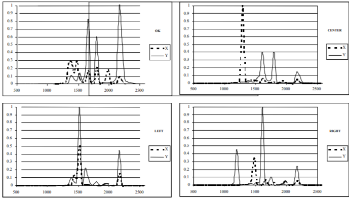
Figure 1. Patterns of normalized stress spectra for the recognized structure states at checkpoints X and Y.

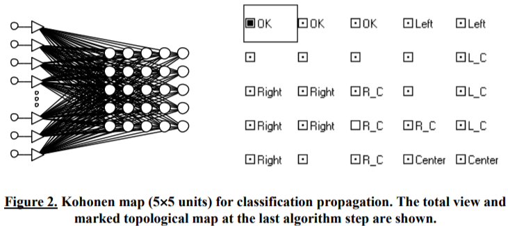
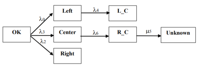
The OK, Center, Left, Right, L_C (Left+Center), R_C (Right+Center) states, which correspond to identified damages, as well as the state Unknown for unknown damages, proved to be necessary for Markov network. To simplify results interpretation, network construction is carried out, firstly, for the six recognizable states, to which the Unknown state is then added.

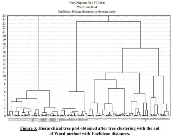
Multivariate clusterization procedure yielded the hierarchical tree plot presented in Figure 3[9]. Taking into account the comments given in Section 2.1.3 reasonable initial clusters forming the model states were estimated with the aid of a tree cross-section at the 5-unit distance. After refining cluster contents via K-means clustering, assigning predominant labels to obtained sets and meshing clusters with identical labels, six higher-level clusters corresponding to the aforementioned damage types (OK, Center, Left, Right, L_C and R_C) were derived. Slight mismatches in distributions of cases over damage clusters are permissible if they do not cause qualitative distortions in a Markov network set of states and their reciprocal connections.

Structure of connections between the recognizable states of Markov network was determined with the aid of Kohonen map consisting of 400 units (Figure 4).

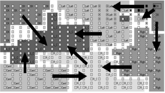
Figure 4. The marked topological map (20x20 units) used to determine connections between Markov network states. Revealed connections are denoted by arrows.

 The shortest distances between neurons of the marked areas are presented in Table 1.

Table 1. The shortest distances between neurons of the marked areas of the topological map (M=2).

Pairs of states, for which the shortest distance was equal to 2, were supposed to be adjacent (k=0). To ascertain directions of transitions between the adjacent states, we took into consideration that the OK state was initial and transitions from this state to the other ones were nonreversible as well as
the facts that the simple damages (Center, Right and Left) preceded more complex ones (R_C and L_C), in which they were included as components. The obtained Markov network with redundant connections is presented in Figure 5.

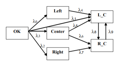
Figure 5. Markov network with redundant connections.

 Taking into account the contiguity of activated areas at the topological map, the network formally included connections between the states R_C and L_C at a given synthesis step in spite of the fact that none of them could be predecessor of another. Record of these connections did not influence the final result since they would be removed later as redundant.

Alternative way of revealing state connections was based on the multidimensional scaling and yielded the 2-D diagram shown in Figure 6[10]. The arrows denote connections determined in accordance with the rules specified in Section 2.1.4. The structure obtained agrees substantially with the results calculated by means of Kohonen maps.

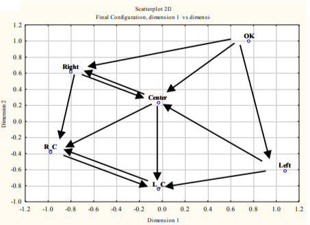
Figure 6. Redundant state connections resulted from multidimensional scaling.

Redundant connections were revealed by comparison of Pearson statistic values obtained by the chi-square minimum method for the complete network shown in Figure 5 and ten reduced networks. In each of these networks, one of 2i (i=0,1,...,9) parameters was supposed to be equal to zero at significance level 0.5. Estimates resulted from the first iteration of network adjustment are shown in Table 2.

Table 2. Statistical estimates resulted from the first iteration of adjustment of Markov network with redundant connections.

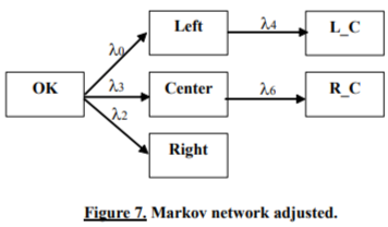
One can see from Table 2 that connections with flow rates h1, h5, h7, h8 and h9 are redundant and may be removed from the network (p>0.5); connections with flow rates h0, h2 and h3 are highly significant and must be retained (p<0.01); connections with flow rates h4, h6 are supposed to be questionable (0.01 <p < 0.5) and must be studied at the following iteration.

The second iteration of adjustment showed that connections with flow rates h4 and h6 are highly significant and must be retained (see Table 3). Markov network obtained is presented in Figure 7.

Table 3. Statistical estimates resulted from the second iteration of adjustment of the Markov network with redundant connections.

The Unknown state was inserted in the network according to the above-mentioned technique, with the exception of adjacency study with the aid of Kohonen map. A network with redundant connections contained all the possible ways of transition to the Unknown state (Figure 8). Removing redundant connections by two iterations of adjustment resulted in a final network presented in Figure 9 (only connection with flow rate turned out to be significant). Kolmogorov set of differential equations describing time-domain dynamics of state probabilities

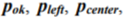
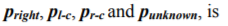
The following initial conditions are given for integration:

Figure 8. Markov network with the Unknown state and redundant connections.

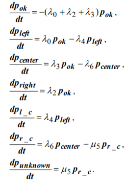
Figure 9. Markov network adjusted (with the Unknown state).

Construction (modification) of a network without adjacency study with the aid of Kohonen network is expedient if the number of free parameters to be found does not exceed the number of independent observed statistics Fk and Kohonen maps are definitely unable to determine the structure of connections (as is the case for the Unknown state).

The synthesized network yields a good forecast: as the probability of exceeding the obtained value 3.396 of the chi-square statistic for six degrees of freedom ((7-1 )x2=12 independent statistics were used to find six free parameters) is 0.76, the chi-square goodness-of-fit test does not give grounds to consider the differences between observed and expected histograms (Figure 10) as statistically significant.

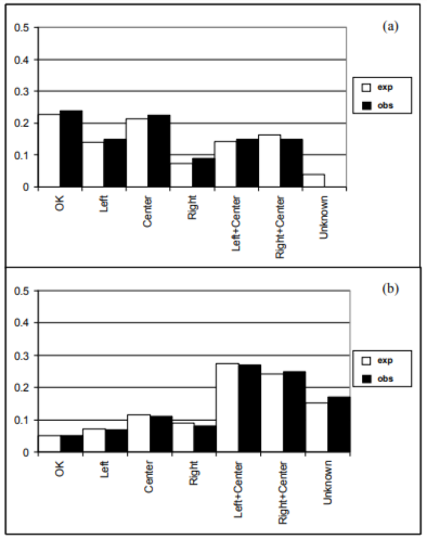
Figure 10. Expected and observed percentage of different damage types appearance after (a) 1000 service hours, (b) 2000 service hours.

Probabilities of different system damages as functions of time are shown in Figure 11. The indicated curves make it possible to forecast the structure service life, establish the justified routine maintenance and facilitate diagnostics.

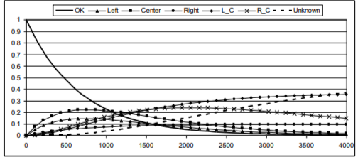
Figure 11. Probabilities of different system damages as functions of time (time is given in hours).

To get the simplest instrument for reproducing the dynamics of damage probabilities, Markov chain for engineering applications was generated from the network presented in Figure 7, by using the technique described in Section 2.3. 100-hour sampling intervals commensurable with 1000-hour damage estimation intervals under consideration were used. Numerical solution of the relevant conditional multivariate optimization problem was computed by means of a special macro implemented at the MS Excel spreadsheet. Residual error resulted from calculations with the sought transition probability matrix was negligible[11]. Markov chain obtained is given in Figure 12. Shown in Figure 13 for illustration is comparison of the integrated Markov network probability functions and simulation results for the corresponding Markov chain after 100 iterations. This simulation was carried out with the aid of the LabVIEW graphical programming environment.

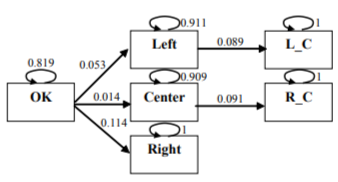
Figure 12. Markov chain with transition probabilities generated from Markov network.

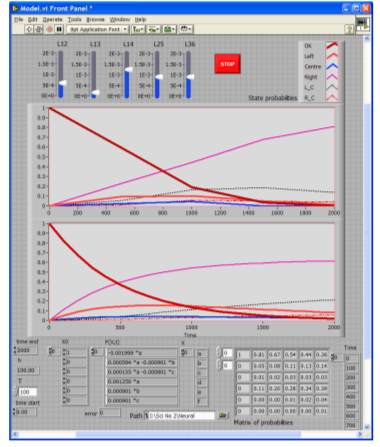
Figure 13. Comparison of the integrated Markov network probability functions (lower plot) and simulation results for the corresponding Markov chain (upper plot) after 100 iterations.

The identification problem was solved to get a sequence of different damages represented by model states, which is most likely occurred, for the sequence of three observed spectral characteristics in structure checkpoints taken with a 100-hour sampling interval. Possible state sequences for the adjusted model shown in the form of Markov network in Figure 7 and in the form of Markov chain in Figure 12 are presented in the second column of Table 4. Table 5 contains parameters of probability density functions for Euclidean distances of observed characteristics arising in case of each state from the corresponding centroids as well as Euclidean distances of observed characteristics from state centroids. To avoid influence of redundant information, the indicated distances were calculated for observed data representation with reduced dimension. According to the problem formulation the system under study starts from the OK state.

Table 4. Possible state sequences for the adjusted model and their probabilistic characteristics.

Table 5. Parameters of normal probability density functions for Euclidean distances of observed characteristics arising in case of each state from the corresponding centroids and Euclidean distances of observed characteristics from state centroids.

Comparison of values presented in the last column of Table 4 yields the following most likely occurred sequence of damages: {OK,Left,Left}.

4.          MAIN RESULTS AND CONCLUSIONS

Methods of construction and analysis of hidden Markov models, which are in the best conformity with observations in case of uncertainties, have been developed. They are based on a novel statistical identification technique and can be applied to both continuous- and discrete-time models.

The model synthesis may be carried out in case of some uncertainties: absence of complete information on system states and their connections is assumed. When solving this problem, a set of relevant states, their connections and optimal values of free parameters of Markov networks are determined. An initial rough model results from either cluster analysis and multidimensional scaling of observed data or their analysis by means of Kohonen maps. Then it suffers proper corrections. Connections between different system states are determined according to contiguity of their clusters or areas of winning units on the topological maps and statistical goodness-of-fit tests. Undefined observed cases are partially identified by the method of classification propagation with the aid of either Kohonen maps or cluster analysis. Histograms of observed frequencies of being in different system states after the given exploitation periods are employed to train the constructed models. Free network parameters are identified by the method of chi-square minimum. In case of models represented by discrete-time structures conversion to continuous-time trained structures is performed to obtain more reliable results with the following return to discrete time and identification of transition probabilities.

Owing to universality and flexibility, the presented way of solution has obvious advantages over the methods used for maximum likelihood estimation of parameters for traditional hidden Markov chains. Moreover, traditional algorithms used for hidden Markov models are unable to solve the applied technical problem considered here when uncertainties with damage types, model states and their connections are the case or the number of sampling points is too small.

The methods suggested are available for specialists responsible for maintenance of technical products. However, these techniques are not fastened to the particular technical problem considered in this paper and can be applied to solve many other technical and non-technical tasks. The obtained Markov models are useful for diagnostics, pattern recognition, structure service lives forecasting and establishing the justified routine maintenance.

Acknowledgements

This work is supported by grant 10-06-00423 from the Russian Foundation for Basic Research.